Scientific Python 5: Enhancing Scientific Writing With Python

Despite being lengthy and obscure, \(\LaTeX\) is still one of the most popular typesetting systems for academic literature. Fortunately, being a compiled (scripting) language, \(\LaTeX\) has a much larger room for customization, and it can do many things that WYSIWYG editors can only dream of. LuaTex is already a very unique and successful attempt to expose the low-level features of the \(\TeX\) compiler to a generic programming language. But due to the prevalence of pdflatex and xetex, I seldom use LuaTex.

There is a very interesting solution, however, that is compatible with all tex compilers and constructs an interface between Python and \(\LaTeX\). It is the \(\LaTeX\) package pythontex. The idea behind pythontex is simple: when you print something with your Python code, instead of writing your outputs to stdout, they are actually redirected to the \(\LaTeX\) document. Accompanied by the Python package PyLaTeX, we can do many amazing things at high efficiency.

Installation and usage of pythontex

The installation of pythontex package varies for different \(\TeX\) distributions. For texlive, the package is probably already installed. For MikTex, it can be installed by the package manager.

The key component of the package is pythontex.py under the package directory (usually it is /texmf/scripts/pythontex). I usually create a symbolic link to this file in my working directory so that I can refer to this file by pythontex.py.

To use the package, first include the package in the preamble, and compile it as usual. After the first compilation, run

python3 pythontex.py (your-document-name).tex --interpreter python:python3

and then recompile the document. In TexStudio, the corresponding build command is:

txs:///pdflatex | python3 pythontex.py %.tex --interpreter python:python3 | txs:///pdflatex

Basic usage of pythontex

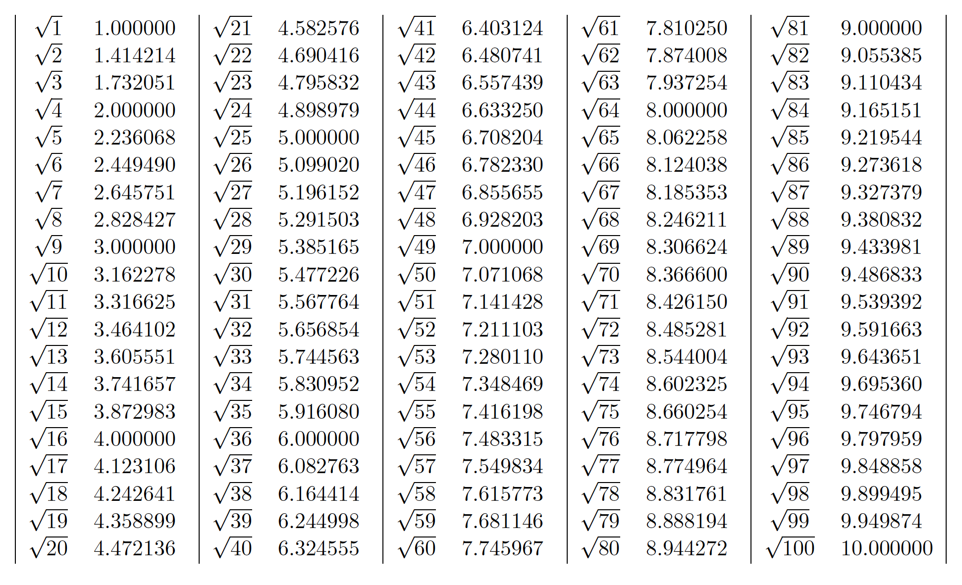
Let’s begin with a simple example to show how pythontex works. Suppose that we would like to create a square root table for integers 1-100. In \(\LaTeX\), we can write the following code:

\documentclass{article}
% I am using article class because pythontex doesn't seem
% to work well with standalone
\usepackage[letterpaper]{geometry}
\usepackage{pythontex}
\begin{document}
\begin{pycode}
from pylatex import Tabular, NoEscape
import math

# the output is gonna be of 20 rows, 10 columns
outArray = [[''] * 10 for _ in range(20)]

# fill in the values
for number in range(1, 101):
    colIndex, rowIndex = divmod(number - 1, 20)
    colIndex *= 2
    # the '$' character should not be escaped
    outArray[rowIndex][colIndex] = NoEscape(r'$\sqrt{%d}$'%number)
    outArray[rowIndex][colIndex + 1] = NoEscape(r'$%4f$'%math.sqrt(number))

# construct table
tabularSpec = '|cp{1.5cm}' * 5 + '|'
tabular = Tabular(tabularSpec)

for rowInd in range(20):
    tabular.add_row(outArray[rowInd])

print(r'\begin{center}')
print(tabular.dumps())
print(r'\end{center}')
\end{pycode}

\end{document}

The code above generates the following output:

It is also possible to refer to python variables within the \(\LaTeX\) document. For example, we have the following array where each element is the natural logarithm of integers 1-10, and we would like to use those values at ease in our document.

import math
arr = [math.log(i) for i in range(1, 11)]

With pythontex, it can be done easily:

\documentclass{article}
\usepackage[letterpaper]{geometry}
\usepackage{pythontex}
\begin{document}
% name this session by "session1"
\begin{pycode}[session1]
import math
arr = [math.log(i) for i in range(1, 11)]
\end{pycode}
The natural logarithm of 4 is \py[session1]{arr[3]}.
\end{document}

The result is shown as below.

Using pythontex and matplotlib to generate beautiful scientific figures rapidly

One advantage of using matplotlib to generate graphs is that it can produce vector graphics, which makes the article’s digital version more readable. However, matplotlib uses san serif font by default, which contradicts with most people’s settings. To cope with this problem, we need to make use of matplotlib’s pgf backend.

Suppose our article uses mathpazo font package, and we want the font of figures to be consistent. We can achieve it with the following code:

import matplotlib
# switch to pgf backend
matplotlib.use('pgf')
# import matplotlib
import matplotlib.pyplot as plt

# update latex preamble
plt.rcParams.update({
    "font.family": "serif",
    "text.usetex": True,
    "pgf.rcfonts": False,
    "pgf.texsystem": 'pdflatex', # default is xetex
    "pgf.preamble": [
         r"\usepackage[T1]{fontenc}",
         r"\usepackage{mathpazo}"
         ]
})

Assume that we have a graphing function as follows:

from scipy.stats import norm
import numpy as np

def GraphNorm(mu, sigmaSqr, filename):
    dist = norm(mu, np.sqrt(sigmaSqr))
    xs = np.linspace(-3.0, 3.0, 100)
    ys = dist.pdf(xs)
    plt.plot(xs, ys)
    plt.ylim((0.0, 0.42))
    plt.title(r'Gaussian ($\mu={},~\sigma^2={}$)'.format(mu, sigmaSqr))
    plt.savefig(filename, bbox_inches='tight')
    # remember to close the figure when using pgf backend
    # otherwise weird things can happen
    plt.close()

With pythontex and PyLaTeX, we can write the code as below:

\documentclass{article}
\usepackage[a4paper, landscape, margin=1in]{geometry}
\usepackage{mathpazo}
\usepackage{pythontex}
\usepackage{graphicx}
\begin{document}

\begin{pycode}
import matplotlib
# switch to pgf backend
matplotlib.use('pgf')
# import matplotlib
import matplotlib.pyplot as plt

# update latex preamble
plt.rcParams.update({
    "font.family": "serif",
    "text.usetex": True,
    "pgf.rcfonts": False,
    "pgf.texsystem": 'pdflatex', # default is xetex
    "pgf.preamble": [
         r"\usepackage[T1]{fontenc}",
         r"\usepackage{mathpazo}"
         ]
})

from scipy.stats import norm
import numpy as np

def GraphNorm(mu, sigmaSqr, filename):
    dist = norm(mu, np.sqrt(sigmaSqr))
    xs = np.linspace(-3.0, 3.0, 100)
    ys = dist.pdf(xs)
    plt.plot(xs, ys)
    plt.ylim((0.0, 0.42))
    plt.title(r'Gaussian ($\mu={},~\sigma^2={}$)'.format(mu, sigmaSqr))
    plt.savefig(filename, bbox_inches='tight')
    # remember to close the figure when using pgf backend
    # otherwise weird things can happen
    plt.close()

graphInfo = [
    (0.0, 1.0, 'fig0.pdf'),
    (1.0, 1.0, 'fig1.pdf'),
    (0.0, 2.0, 'fig2.pdf'),
    (1.0, 2.5, 'fig3.pdf')
]

# generate the graphs
for info in graphInfo:
    GraphNorm(*info)


from pylatex import Figure, NoEscape

filenameFormat = 'fig{}.pdf'
# compute line width
lineWidthStr = NoEscape(r'{}\linewidth'.format(1.0 / len(graphInfo) * 0.9))

# create figure
figure = Figure(position='htpb')
for i in range(len(graphInfo)):
    figure.add_image(filenameFormat.format(i), width=lineWidthStr)

print(figure.dumps())

\end{pycode}
\begin{center}
\large Gaussian $\mu$ $\sigma^2$ 1234567890
\end{center}
\end{document}

It generates the following output:

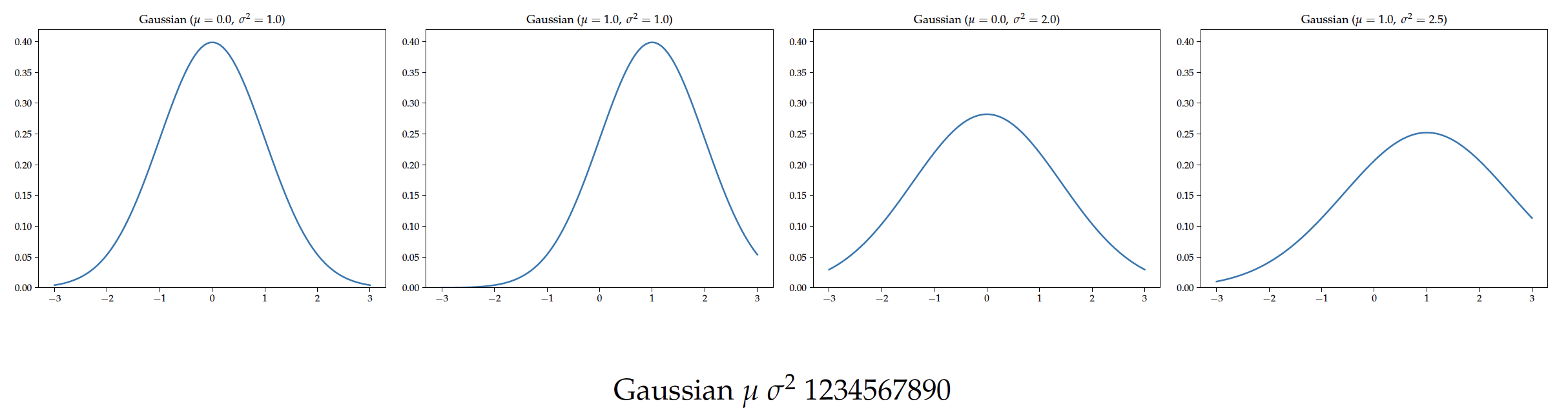
We can see that now the style of text in the article is the same as the style in figures. Notice how we create these figures in batch. Just by changing several lines of code, we can create completely different figures. It is extremely convenient for those researchers who need to change his/her drafts frequently.