Spherical Projection Correction

In this article I briefly discussed and demonstrated how to simulate projecting images onto a spherical screen with a normal projector. Now, the problem comes naturally: how do we correct the image so that it looks right? By modifying the PyOpenGL program slightly, we can have a image generator that can help us analyze this problem and formulate a solution.

Addressing the problem conceptually

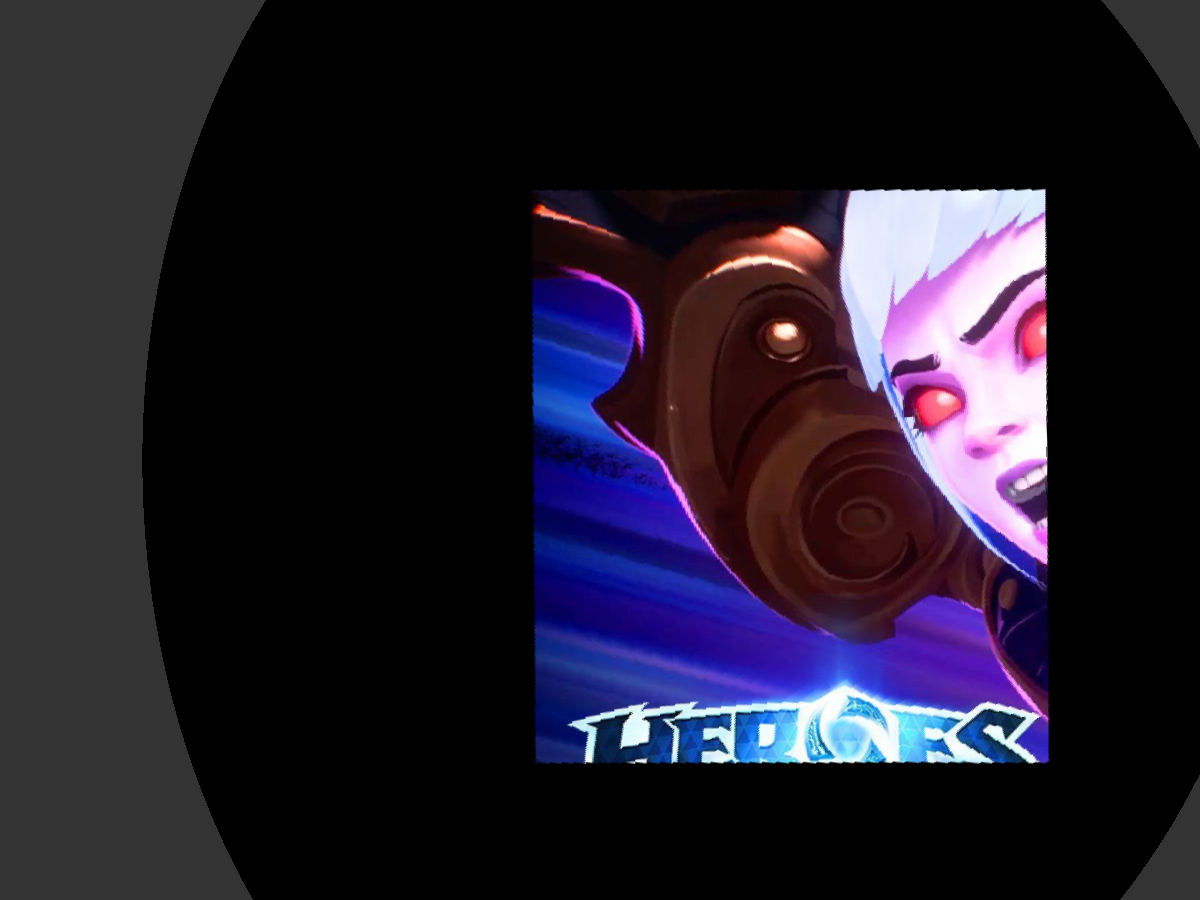
Assume that the projector is presenting the image on the left (a.k.a. source image), and from the observer’s point of view, he/she is getting the image on the right (a.k.a. receiving image).

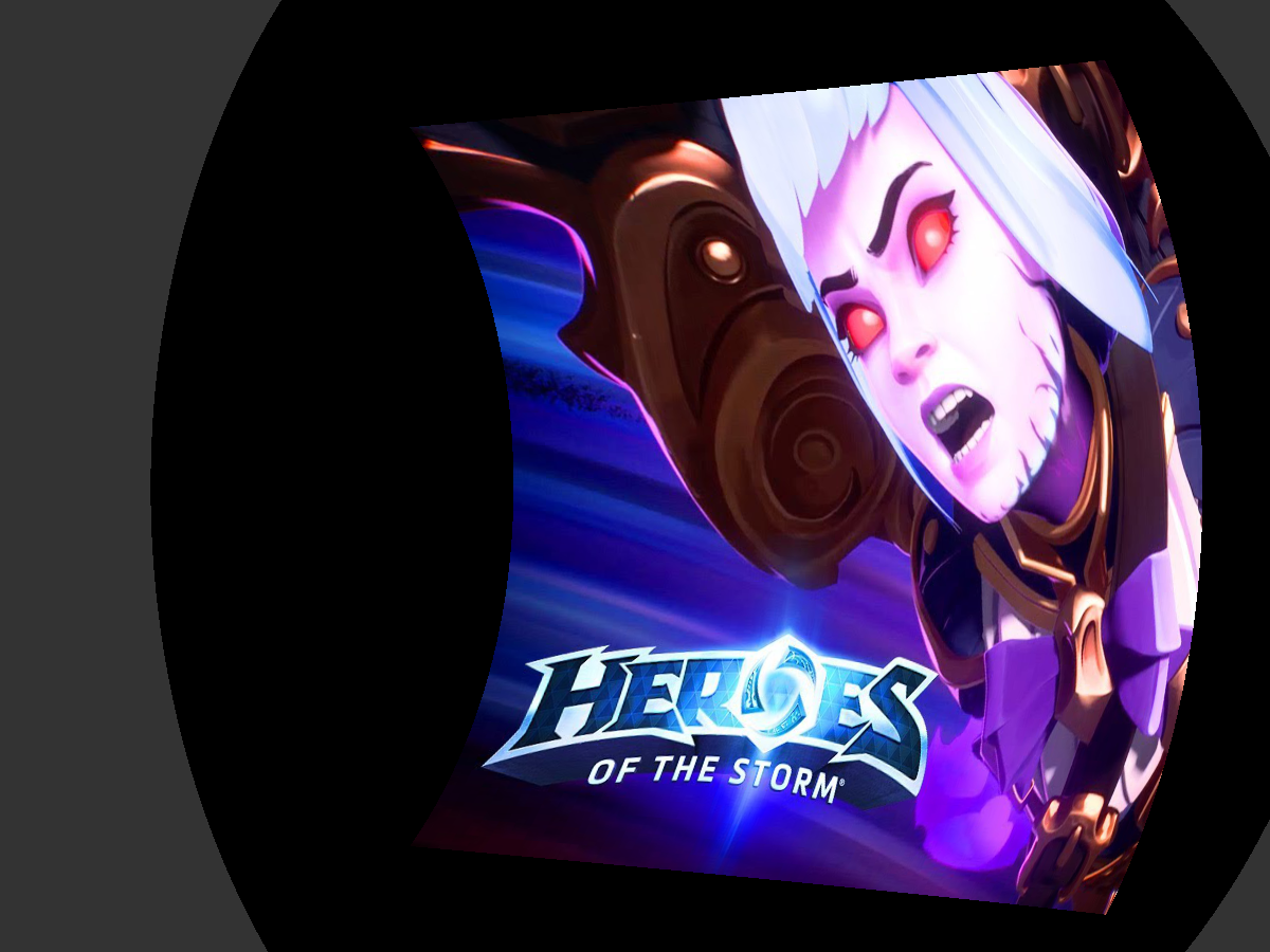
Our first observation is that not all parts of the source image is visible on the receiving image. The pixels on the receiving image that are influenced by the projector forms receiving region. The pixels on the source image that forms the receiving region constitute source region. If we assume that the image is continuous (i.e. with infinite number of pixels), then it can be seen that for each pixel in the source region, there is a corresponding pixel in the receiving region, and vice versa. If we can find this positional correlation, we can surely generate a source image that allows us to output a normal image on the spherical screen.

As a matter of fact, the method introduced in the PyOpenGL article is exactly one of the ways to determine this correlation. However, in order to use that method to correct the image, one needs to gauge the orientations, positions of the projector and camera very precisely, which can be costly. It would be really convenient if we can find a way to correct the image just with a projector and a camera (which generates the receiving image).

An interactive method using linear approximation

Since it is a purely positional mapping, we can use a set of linear functions to approximate the actual mapping. In order to do this, we can let the projector present a set of points (a.k.a. calibration points) on the screen and record their projected position on the spherical screen.

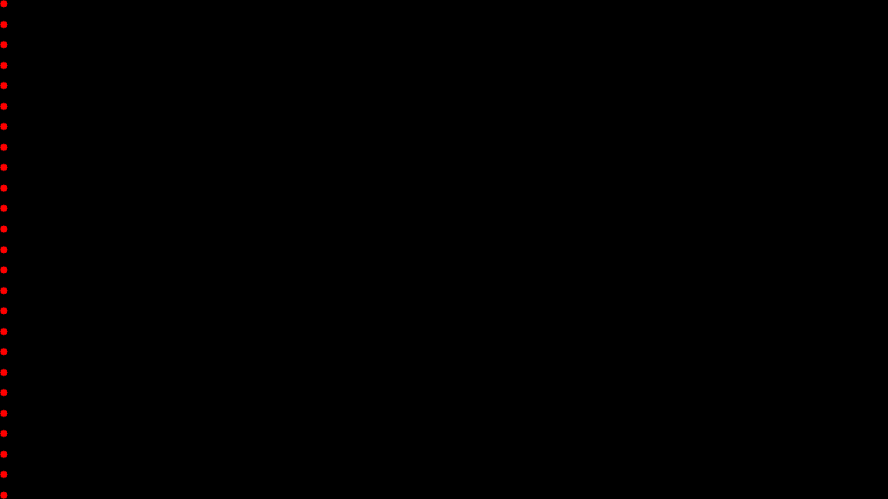
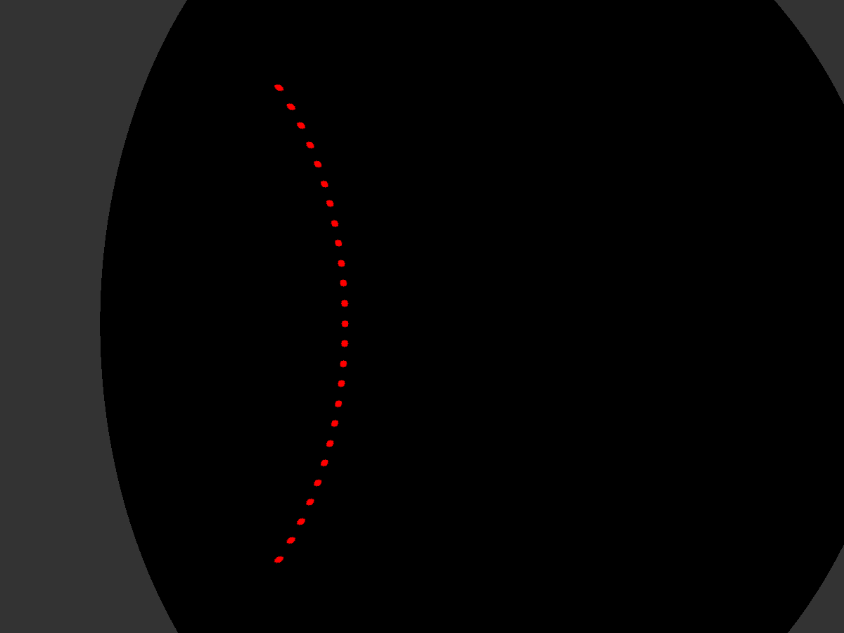
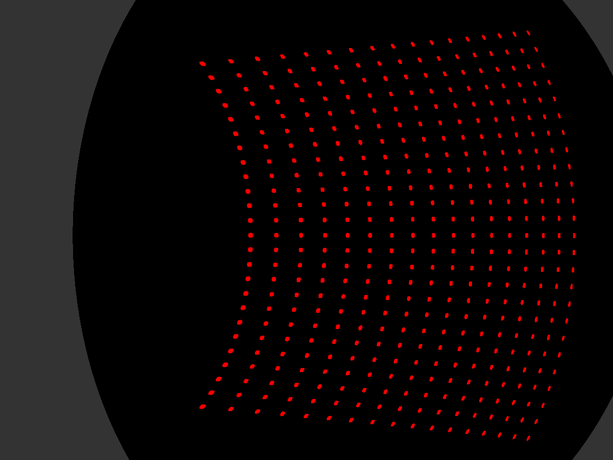
Now for a calibration point in source image space (which is inside the source region), it has a corresponding point in the receiving image space. These uniformly distributed points form a grid on both image spaces, and we can use a linear relation to approximate the translation between two grids.

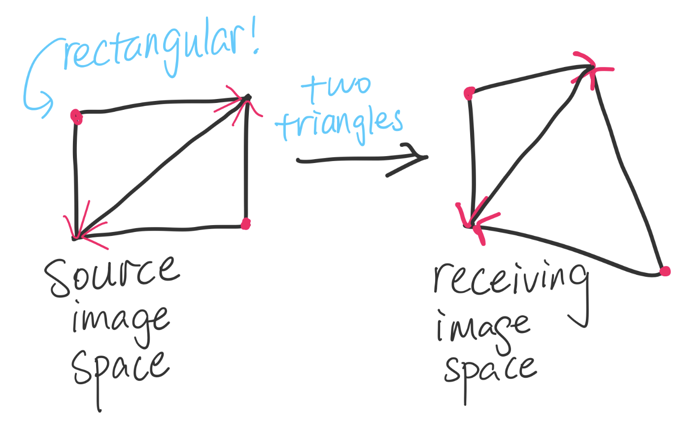
Since the math for this conversion is rather trivial, I am not elaborating on it. All the concepts are explained pretty clear in the figure above.

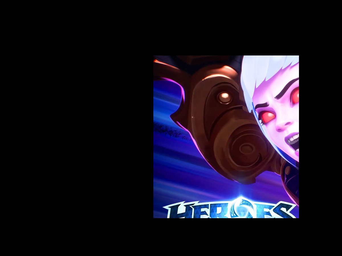
In order to present a normal image on the screen, we construct a blank image whose size is identical to the receiving image, which is called the reference image. Then we select a rectangular box inside the receiving region and fill it with the image we want to show. An example is shown as below.

Now we can start to build our new source image. With the linear mapping we determined before, we are able to compute the corresponding point in the receiving region for each point in the source region on the new source image. Then we can assign the color of that point on the source image with the corresponding color on the reference image. To make the color smoother, I use bilinear interpolation in this step. The result is shown as below.

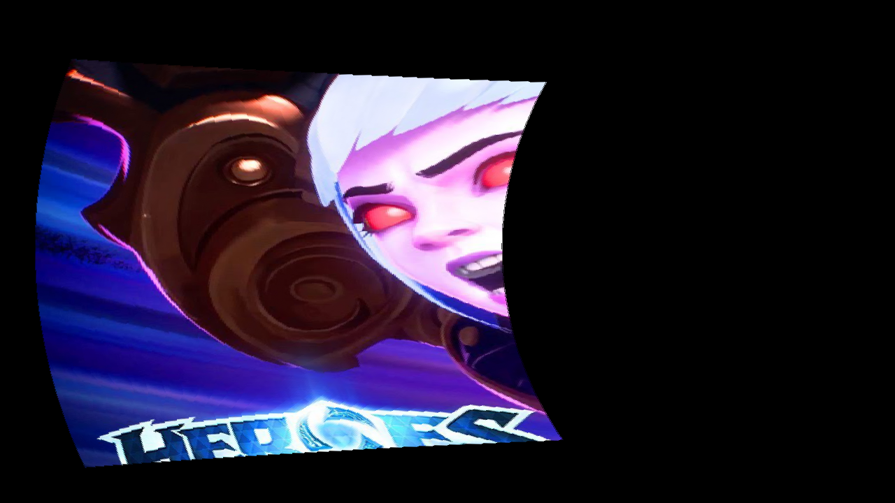
This method is much more practical since we only need a camera and a computer, alongside with the projector to achieve projection correction.

Demo

The demo of this article can be found on github. To run it, execute main.py. The program will generate images with calibration points and use them to interact with the PyOpenGL based image generator. Once the receiving region is determined, one will be asked to select a rectangular region inside it.

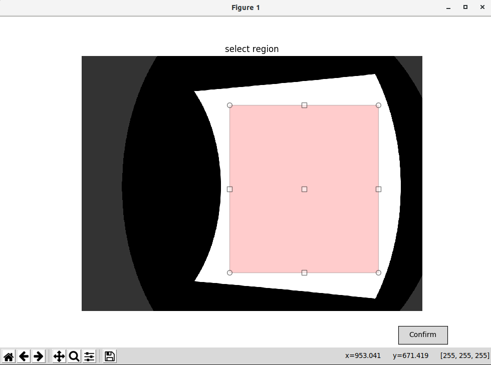
After selecting the region, one can press the Confirm button to proceed (moving the cursor onto the button may cause the rectangular box to disappear, but it does not affect the outcome). If the selection is invalid, the figure will keep appearing until a valid one is provided. The program will continue to compute the new source image and receiving image, and then present the results to the screen. Considering the loop efficiency of Python, it may take a while until the images are ready.