Performance Evaluation Issues in Image Forensics

20 Feb 2020

We observed the fact that, in recent literature, the performance of tampering localization techniques are evaluated by rather universal metrics, such as accuracy, ROC curve, AUC, F-score and so on. These metrics are designed for binary classification problems where individual samples are independent. However, it is easy to see that in the case of image tampering localization, the image patches (pixels) that are fed into the classifier do not follow the metrics’ design. As it will be shown in this article, these metrics not very descriptive when applied to image tampering detection practice.

Tampering Localization, Performance Evaluation and Human Perception

Due to the complexity of image tampering localization problem, it is very unlikely for the user of an automatic image tampering localization system to consider its results as a final decision. That is to say, such systems usually serve as an assistance to allow human inspectors to make better judgments. Usually the localization is done at patch level, where a patch is a small region (say, 10 × 10) extracted from a rectangular grid in the image.

It is also possible to achieve localization at pixel level, which has a smaller granularity and therefore higher precision, but there is little difference between these two approaches essentially. It can be seen that the patch level approach is less accurate, but it is more commonly used because a patch of image contains more statistical features and reduces the dimensionality of image data (because there are less patches than pixels). For simplicity, in the subsequent discussion, we assume that the localization is done at patch level.

In recent literature, authors usually use general purpose machine learning performance evaluation metrics to assess the effectiveness of image tampering localization methods. The commonly used metrics include accuracy, AUC and F-score. However, the image tampering localization scenario is different from normal binary classification problems for the following reasons:

1. A single image contains an enormous amount of inputs, whose outputs need to be inspected as a whole
2. The inputs to the tampering localization classifier are not independent
3. The goal of tampering localization is to generate human perceivable results

These factors render these metrics less reflective in tampering localization scenario. Or at least their values should be interpreted in a different manner. For reference, we briefly introduce the concepts in performance evaluation below:

(Concepts from confusion matrix: \(TP\): true positive, \(TN\): true negative, \(FP\): false positive, \(FN\): false negative, \(P\): all positive, \(N\): all negative.)

• $\mbox{recall}=\frac{TP}{P} = \frac{TP}{TP+FN}$
• $\mbox{fall-out}=\frac{FP}{N}=\frac{FP}{FP+TN}$
• $\mbox{precision}=\frac{TP}{TP+FP}$
• $\mbox{accuracy} = \frac{TP+TN}{P+N} = \frac{TP+TN}{TP+TN+FP+FN}$
• $\mbox{F-score} = 2 \cdot \frac{\mbox{precision} \cdot \mbox{recall}}{\mbox{precision} + \mbox{recall}} = \frac{2TP}{2TP+FP+FN}$
• The ROC curve is created by plotting the recall against the fall-out at various threshold settings.
• The Area Under the Curve (AUC) is the area under the ROC curve.

Generation of Hypothetical Predicted Mask

We would like to show that the decline of metric effectiveness is not bond to specific classifier. In fact, it is due to the the limitation of performance metrics themselves as they are not designed for this scenario. In order to demonstrate how ubiquitous the problem is, we devise a way to randomly generate predicted masks based on a given performance metric, which can yield the \emph{bad cases} we want at high probability. In all the following examples, it is assumed that the ground truth mask is already known. To show the different visual perception effects of distinctive shapes in masks, we apply the evaluation on several different predefined pixel level masks, which are the illustrated in the figure below. There corresponding patch level masks can be acquired easily and therefore are not attached.

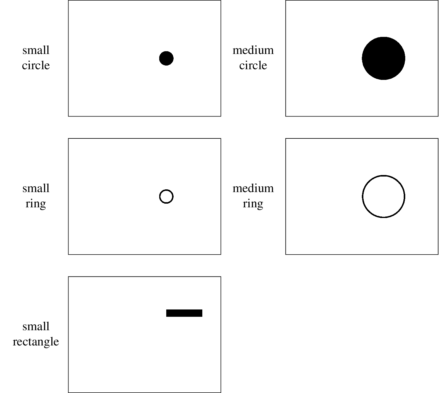
For the subsequent discussion, the ground truth mask will be denoted by \(g\), where the value on \(i\)th row, \(j\)th column is given by

\[\begin{align*} g(i, j) = \begin{cases} 0, &\mbox{if the patch is genuine}\\ 1, &\mbox{if the patch is tampered}. \end{cases} \end{align*}\]

In our illustrations, \(g(i, j) = 0\) is shown by white patches, while \(g(i, j) = 1\) is shown by black patches. The hypothetical predicted mask will be denoted by \(h\), which can take on both binary values or real values on \([0, 1]\) depending on the context. It can be clearly seen that \(h\) has the same dimensionality as \(g\).

Generate hypothetical predicted mask given accuracy

It is relatively simple to generate a hypothetical predicted mask \(h\) given an accuracy value \(a\). In the scenario, \(h\) only needs to take on binary values. To generate \(h\), we can sample from a Bernoulli distribution \(\mathcal{B}(p, q)\), where \(p = a\) and \(q = 1-a\). The algorithm is shown as below.

\begin{algorithm}
\begin{algorithmic}

\PROCEDURE{get-h-given-acc}{$g, a$}
\STATE $p = a, q = 1-a$

  \FOR{\textbf{each} possible $(i, j)$ pair}
      \STATE sample a value $v$ from $\mathcal{B}(p, q)$
      \IF{$v = 1$}
        \STATE $h(i, j) = g(i, j)$
        \ELSE
        \STATE $h(i, j) = 1 - g(i, j)$ \COMMENT{equivalent to flipping the binary bit}
      \ENDIF
  \ENDFOR
  \RETURN $h$

\ENDPROCEDURE
\end{algorithmic}
\caption{Generate $h$ given accuracy $a$}
\end{algorithm}

It is easy to see why \(h\) will have accuracy \(a\) approximately, because the event of \(h(i, j)\) being assigned with a correct value has a probability of \(p = a\).

Generate hypothetical predicted mask given AUC

Because the AUC implies a huge degree of freedom, given an AUC value \(u\), it is difficult to enumerate all possible ROC curves, which may lead to different visual effects. As our purpose is to create an illustration that loosely represents the given AUC value, we would like to make the following assumptions to make the problem more tractable:

1. When the AUC is high, the shapes of ROC curves tend to look alike and therefore can be approximated by a family of curves.
2. Suppose an ROC curve is uniformly discretized into a set of points \(P = \{p_1, p_2, \ldots, p_n\}\), where \(P\) is well-sorted by their spatial occurrence from the top right corner to the bottom left corner. We assume that the threshold values are also uniformed distributed (by the length of the ROC curve) from 0 to 1 on these \(n\) points.

The family of curves that is chosen for ROC curve approximation is a simple 3-line-segment scheme. The equation of the first line segment is given by \(l_1: y = kx\), where \(k \geq 1\) is the gradient. Because the ROC curve is constrained in a square box, it can be seen that \(l_1\) intersects with the \((0, 1)\rightarrow(1, 0)\) diagonal at \(p(\frac{1}{k + 1}, \frac{k}{k + 1})\). We would like to scale the line segment between the origin and \(p\) by a factor of \(1 - \frac{1}{2k}\). The second line segment is the symmetry of the first line segment about the same diagonal, and the third line segment connects the previous two line segments. It can be expressed as the piecewise function below:

\[\begin{align*} f(x) = \begin{cases} kx, & 0 \leq x < \frac{k - \frac{1}{2}}{k \left(k + 1\right)}\\ \frac{k x \left(k + 1\right) + \frac{k \left(2 k - 1\right)}{2} - k + \frac{1}{2}}{k \left(k + 1\right)}, & \frac{k - \frac{1}{2}}{k \left(k + 1\right)} \leq x < \frac{3}{2 \left(k + 1\right)}\\ \frac{k + x - 1}{k}, & \frac{3}{2 \left(k + 1\right)} \leq x \leq 1. \end{cases} \end{align*}\]

Because the shape of the curve are completely determined by the choice of \(k\), for simplicity, we shall call it a \(k\)-ROC curve. Different \(k\)-ROC curves and their corresponding AUC values are shown as below.

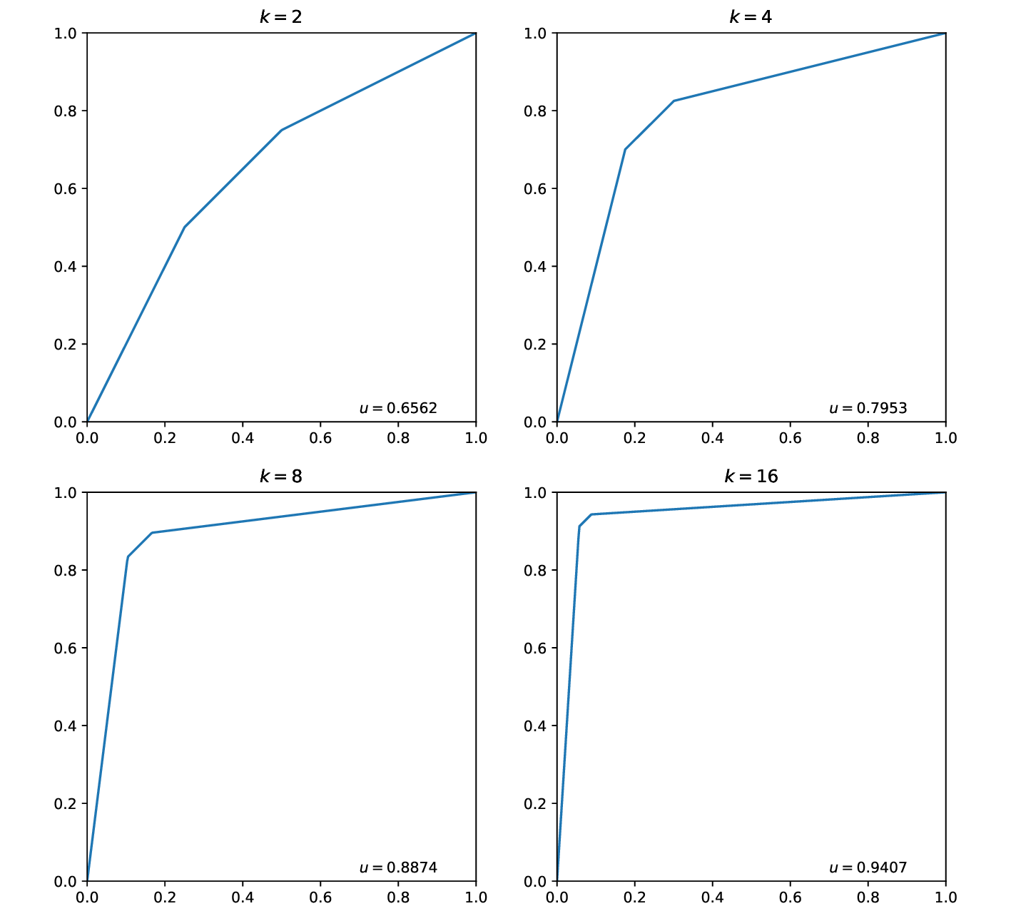
When \(k \rightarrow +\infty\), because \(\lim_{k \rightarrow +\infty} 1 - \frac{1}{2k} = 1\), \(p\) and its symmetry will both be close to \((0, 1)\). Therefore, it is easy to see that when \(k \rightarrow +\infty\), \(u \rightarrow 1\).

The relationship between \(k\) and \(u\) is given by

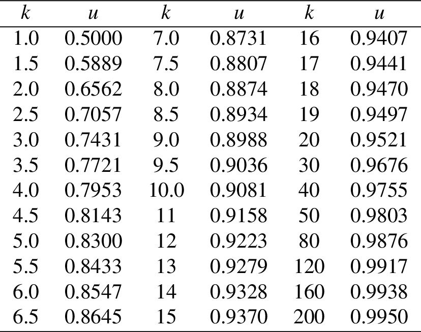
\[\begin{align*} u = \frac{8 k^{3} - k + 1}{8 k^{2} \left(k + 1\right)}. \end{align*}\]

Because it is nontrivial to solve for \(k\) given \(u\), a \(k-u\) table is attached to help one select a nearest \(k\) value given \(u\), which is shown as below.

\(\require{newcommand}\newcommand{\rocpos}{\operatorname{rocpos}}\newcommand{\roclen}{\operatorname{roclen}}\) We also need to parameterize the \(k\)-ROC curve into \(t \in [0, 1]\) by its length, where \(t = 0\) indicates the bottom left corner and \(t = 1\) indicates the top right corner. More specifically, we need to determine a function \(\rocpos(k, t)\) that returns the Cartesian coordinate of the parameter \(t\) on the curve. Since \(k \geq 1\), it is easy to compute that the length of the first line segment, denoted by \(\roclen_1(k)\), is

\[\begin{align*} \roclen_1(k) = \frac{(2k-1)\sqrt{k^2 + 1}}{2k(k+1)}. \end{align*}\]

The length of the second line segment equals to the first, and the length of the third line segment, denoted by \(\roclen_3(k)\), is

\[\begin{align*} \roclen_3(k) = \frac{\sqrt{2}}{2k}. \end{align*}\]

Denote the total length of a \(k\)-ROC curve by \(\roclen(k)\), it can be seen that

\[\begin{align*} \roclen(k) = 2 \cdot \roclen_1(k) + \roclen_3. \end{align*}\]

By interpolating the segments linearly, we can see that the relationship between the \(x\) component of Cartesian coordinate and \(t\) is as follows:

1. If \(0 \leq t < \frac{\roclen_1(k)}{\roclen(k)}\), then

   \[\begin{align*} x = \left[ t \middle/ \frac{\roclen_1(k)}{\roclen(k)}\right] \cdot \frac{k - \frac{1}{2}}{k \left(k + 1\right)}. \end{align*}\]

2. If \(\frac{\roclen_1(k)}{\roclen(k)} \leq t < \frac{\roclen_1(k) + \roclen_3(k)}{\roclen(k)}\), then

   \[\begin{align*} x = \frac{k - \frac{1}{2}}{k \left(k + 1\right)} + \left[ \left(t - \frac{\roclen_1(k)}{\roclen(k)} \right) \middle/ \frac{\roclen_3(k)}{\roclen(k)}\right] \cdot \left[ \frac{3}{2 \left(k + 1\right)} - \frac{k - \frac{1}{2}}{k \left(k + 1\right)} \right]. \end{align*}\]

3. If \(\frac{\roclen_1(k) + \roclen_3(k)}{\roclen(k)} \leq t \leq 1\), then

   \[\begin{align*} x = \frac{3}{2 \left(k + 1\right)} + \left[ \left(t - \frac{\roclen_1(k) + \roclen_3(k)}{\roclen(k)} \right) \middle/ \frac{\roclen_1(k)}{\roclen(k)}\right] \cdot \left[ 1 - \frac{3}{2 \left(k + 1\right)} \right]. \end{align*}\]

It can be seen that \(\rocpos(k, t) = (x, f(x))\). Now we can generate \(h\) given \(k\) and \(n\) with the algorithm below.

\begin{algorithm}
\begin{algorithmic}

\PROCEDURE{get-h-given-auc}{$g, k, n$}
\STATE\COMMENT{assume $n > 1$}
\STATE $thrs=~$array of $n$ evenly spaced numbers over $[0, 1]$
\STATE $pos=~$indices of all positive samples in $g$
\STATE $neg=~$indices of all negative samples in $g$
\STATE randomly shuffle $pos$ and $neg$
\FOR{$i=0$ \textbf{to} $n-2$}

  \STATE  $fpr_i, tpr_i = \operatorname{rocpos}(k, 1 - thrs[i])$
  \STATE $fpr_{i}, tpr_{i + 1} = \operatorname{rocpos}(k, 1 - thrs[i + 1])$
  \STATE\COMMENT{the following values are computed according to the fpr/tpr values above}
  \STATE $tp_i, fp_i=~$ number of true positive/false positive samples at $thr[i]$
  \STATE $tp_{i + 1}, fp_{i + 1}=~$ number of true positive/false positive samples at $thr[i + 1]$
  \STATE $thr = (thrs[i] + thrs[i + 1]) / 2$ \COMMENT{threshold now}
  \FOR{$j = 1$ \textbf{to} $tp_{i + 1} - tp_{i}$}
    \STATE $ind=~$the first item popped from $pos$
    \STATE $h(ind) = thr$
  \ENDFOR
  \FOR{$j = 1$ \textbf{to} $fp_{i + 1} - fp_{i}$}
    \STATE $ind=~$the first item popped from $neg$
    \STATE $h(ind) = thr$
  \ENDFOR
\ENDFOR

\RETURN $h$

\ENDPROCEDURE
\end{algorithmic}
\caption{Generate $h$ given $k$ and $n$}
\end{algorithm}

This algorithm can indeed generate \(h\) that has a \(k\)-ROC curve, because as the \(fpr\) and \(tpr\) changes between two points of the \(k\)-ROC curve, the algorithm assigns patches with certain values so that the \(fpr\) and \(tpr\) of \(h\) will change in the same way. Once the ROC curve of \(h\) follows the \(k\)-ROC curve, \(h\) will also have the AUC value defined by the \(k\)-ROC curve.

Observations

Big gap in metrics may lead to similar performance in practice

This image shows the the hypothetical output maps given particular accuracy scores.

The image shows the hypothetical output maps given particular \(k\) values, where each value of \(k\) corresponds to an AUC score.

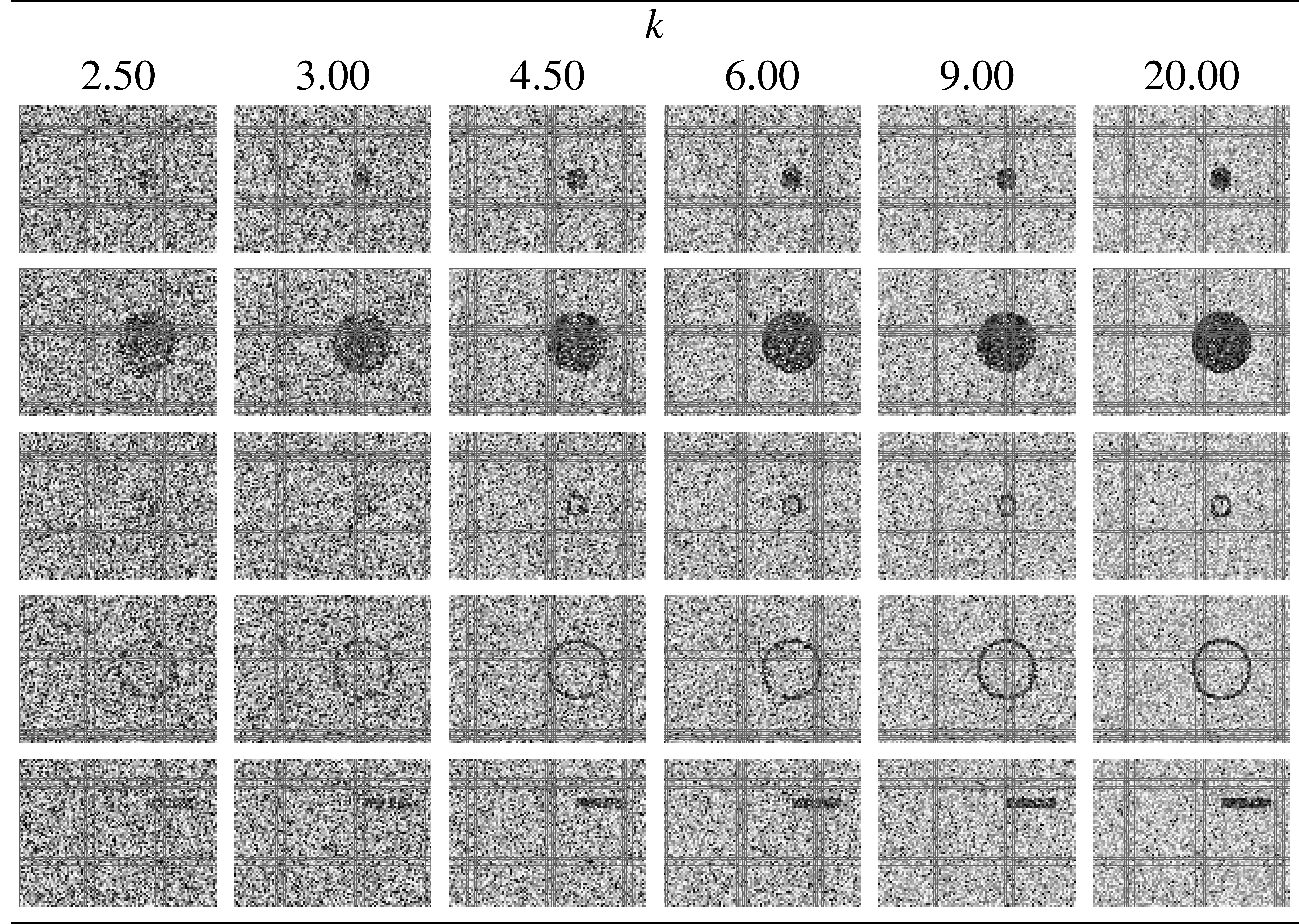
It can be seen that objects are observable in some output maps with lower metric scores.

Methods with lower metrics may work better

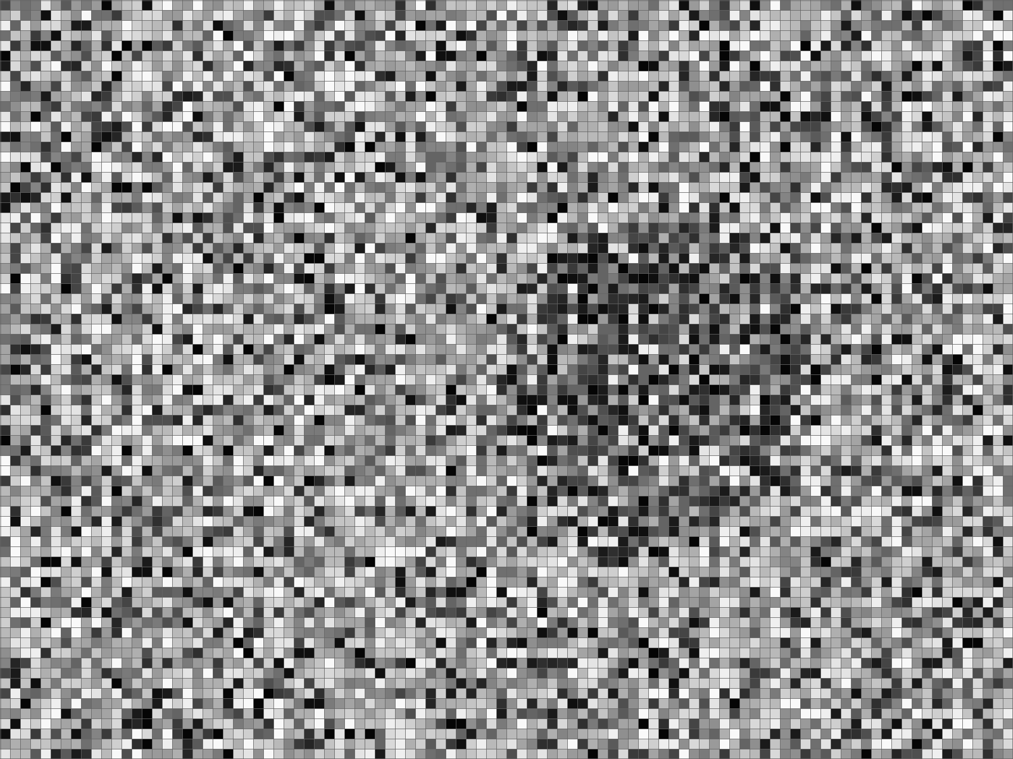
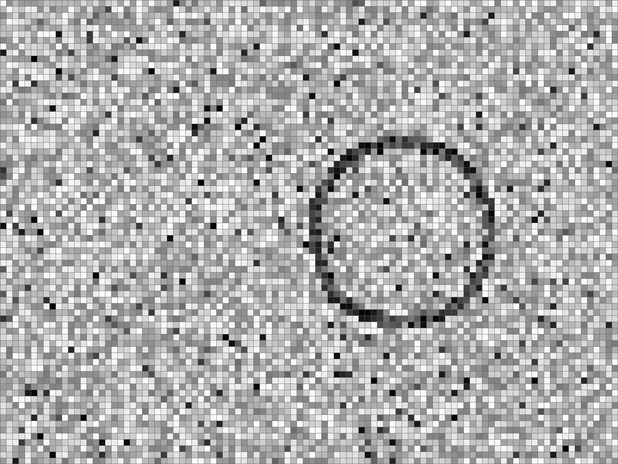
It is pointed out by Zhou et al.¹ that the edges of the tampered region are easier to detect because the statistical patterns change greatly there. What if there is a classifier that is very sensitive to the edges of the tampered region but not the inner? For example, assume that the tampered region is given by medium circle in mask templates. The outputs of classifier \(A\) and \(B\) are shown as below. If we compute the AUC of classifier \(B\), the value is only around 0.62, which is lower than the output of classifier \(A\), which has an AUC of approximately 0.70. However, the shape of tampered region is much clearer in the output of classifier \(B\). That is to say, output maps with lower AUC values may look better for humans.