LaTeX3: Programming in LaTeX with Ease

Many people view LaTeX as a typesetting language and overlook the importance of programming in document generation process. As a matter of fact, many large and structural documents can benefit from a programming backend, which enhances layout standardization, symbol coherence, editing speed and many other aspects. Despite the fact the standard LaTeX (LaTeX2e) is already Turing complete, which means it is capable of solving any programming task, the design of many programming interfaces is highly inconsistent due to compatibility considerations. This makes programming with LaTeX2e very challenging and tedious, even for seasoned computer programmers.

To make programming in LaTeX easier, the LaTeX3 interface is introduced, which aims to provide modern-programming-language-like syntax and library for LaTeX programmers. Unfortunately, there is little material regarding this wonderful language. When I started learning it, I had to go through its complex technical manual, which is time-consuming. Therefore, I decide to write a LaTeX3 tutorial that is easy-to-understand for generic programmers.

Preface
Why LaTeX3?
LaTeX3 Naming Conventions (I-1)
Reading LaTeX3 Documentation
Functions & Variables
Macro Expansion Control (V)
LaTeX3: Token List and String
- Token list (VII)
  - Constructing a command in token list
  - Student management system
- String (VIII)
  - Vertical text node in TikZ
LaTeX3: Numeric Evaluation and Boolean Logic
LaTeX3: Data Structure
- Queue (X, XV)
  - Student management system
  - Bracket matching
- Dictionary (XVII)
  - Arabic numerals to English (0-99)
LaTeX3: Regular Expression (XXVIII)
LaTeX3: File I/O (XIX)
- Writing to a file
- Reading and parsing comma-separated file
Memo
End Note

Preface

The preamble of all examples
```
\documentclass{article}
\usepackage[T1]{fontenc}
\usepackage{tikz} % load TikZ for some examples
\usepackage{expl3} % load latex3 packages
\usepackage{xparse}
```
Please place the example content between \begin{document} and \end{document} blocks. Note that in newer $\text{[math]}$ distributions (later than 2020-02-02 release), expl3 has become part of $LaTeX2e$ as the “L3 programming layer”. In these new distributions, there is no need to use expl3 package explicitly.
All $LaTeX3$ examples have been tested with TeXLive 2020 (Windows 10)
This article only provides simple introduction to frequently used $LaTeX3$ modules, because it is fairly difficult for me to cover all aspects of $LaTeX3$ within a short amount of time. For now, all $LaTeX3$ APIs are documented in The LaTeX3 Interfaces.
The roman letters in section titles are the corresponding chapter numbers in The LaTeX3 Interfaces.

Why LaTeX3?

Handle macro expansion like a boss

Fundamentally, $\text{[math]}$ works by doing macro substitution: commands are substituted by their definition, which is subsequently replaced by definition’s definition, until something irreplaceable is reached (e.g. text). For example, in the following example, \myname is substituted by \mynameb; \mynameb is then substituted by \mynama; and eventually, \mynamea is replaced by John Doe, which cannot be expanded anymore. This process is called expansion.

\newcommand{\mynamea}{John Doe}
\newcommand{\mynameb}{\mynamea}
\newcommand{\myname}{\mynameb}
My name is \myname.

Most $\text{[math]}$ command we use everyday has complicated definitions. During compilation, they will be expanded recursively until text or $\text{[math]}$ primitive is reached. This process sounds pretty straightforward, until we want to change the order of macro expansion.

Why do we need to change the order of macro expansion? Let’s consider the \uppercase macro in $LaTeX2e$ , which turns lowercase letters into uppercase ones. But consider the following case, where we try to apply \uppercase to letters abcd and a command \cmda. Since \cmda expands to abcd, we expect the outcome to be ABCDABCD. In reality, $\text{[math]}$ gives us ABCDabcd, which means the content of \cmda is unchanged.

\newcommand{\cmda}{abcd}
\uppercase{abcd\cmda} %ABCDabcd

How can this happen? During the expansion of \uppercase, the command scans the item inside the adjacent curly braces one by one. If an English letter is encountered, an uppercase counterpart is left in the output stream; otherwise, the original item is left in the input stream. When it’s \cmda’s turn, because it is a command instead of a letter, it is left untouched in the output stream, which is expanded to abcd later.

What if we want to capitalize everything inside the curly braces? That would require the macro \cmda to be expanded before \uppercase, or equivalently, changing the order of macro expansion. The classical way of doing so in $\text{[math]}$ is via \expandafter. Unfortunately, the usage of \expandafter is extremely complicated¹: in a string of n tokens², to expand the ith token, there must be $2^{n-i}-1$ \expandafter’s before the ith token. Below is a example of how bad this can look like:

\documentclass{article}
\begin{document}

\def\x#1#2#3#4{%
  \def\arga{#2}%
  \def\argb{#3}%
  \def\argc{#4}%
  \expandafter\expandafter\expandafter\expandafter\expandafter\expandafter\expandafter#1%
    \expandafter\expandafter\expandafter\expandafter\expandafter\expandafter\expandafter
      {\expandafter\expandafter\expandafter\arga\expandafter\expandafter\expandafter}%
        \expandafter\expandafter\expandafter{\expandafter\argb\expandafter}\expandafter
          {\argc}}

\def\y#1#2#3{\detokenize{#1#2#3}}

\x\y{arg1}{arg2}{arg3}

\end{document}

Clearly, it is nowhere near decency: the excessive number of \expandafter’s are sometimes referred to as “\expandafter purgatory”. As a result, one of the features of $LaTeX3$ is to provide simple and reliable expansion control.

Messy interfaces in LaTeX

Believe it or not, $\text{[math]}$ is able to achieve everything other generic programming languages can do (e.g. C++, Python, Java)³. However, the function call conventions can be wildly distinct across different tasks; some similar functionalities can be independently implemented various packages. Here are some examples:

File read

\newread\file
\openin\file=myfilename.txt
\loop\unless\ifeof\file
    \read\file to\fileline % Reads a line of the file into \fileline
    % Do something with \fileline
\repeat
\closein\file

File write

\newwrite\file
\immediate\openout\file=myfilename.txt
\immediate\write\file{A line of text to write to the file}
\immediate\write\file{Another line of text to write to the file}
\closeout\file

Integer arithmetic

\newcount\mycount
\mycount=\numexpr(25+5)/3\relax
\advance\mycount by -3
\multiply\mycount by 2

Condition

% command-related if statement
\ifx\mycmd\undefined
undefed
\else
  \if\mycmd1
  defed, 1
  \else
  defed
  \fi
\fi

% number-related if statement
\ifdim#1pt=#2pt
    Equal.\\
\else%
    Not equal.\\
\fi%

Loop

% use \loop
\newcount\foo
\foo=10
\loop
  \message{\the\foo}
  \advance \foo -1
\ifnum \foo>0
\repeat

% while loop (provided by `ifthen` package)
\newcounter{ct}
\setcounter{ct}{1}
\whiledo {\value{ct} < 5}%
{
  \the\ct
  \stepcounter {ct}%
}

% for loop (provided by `ifthen` package)
\forloop{ct}{1}{\value{ct} < 5}%
{%
  \the\ct
}

These inconsistencies set a high bar for new $\text{[math]}$ users and make it difficult to connect multiple components together, even for experienced $\text{[math]}$ programmers. Therefore, $LaTeX3$ aims to provide standardized programming interfaces and documentation for the language.

Goals of LaTeX3

Modernize the syntax of $\text{[math]}$
Simplify macro expansion control
Unify the interfaces across various components
Provide standardized libraries for $\text{[math]}$ packages (e.g. floating-point arithmetic, regular expression, random number, high-performance array, etc.)

LaTeX3 Naming Conventions (I-1)

In the following code snippet, we declare a variable \vara and a function \cmda. The way we distinguish between a variable and a function is simply by judging whether the command absorbs arguments or not. However, the fact that they are all called “commands” and created with \newcommand reflects that they are fundamentally the same for $\text{[math]}$ system.

\newcommand{\vara}{this is a variable}
\newcommand{\cmda}[1]{this is a command: #1}

From users’ perspective, it is important to separate variables from functions because their usages are different. Therefore, our only option is to encode this information into the name of commands, so that users can differentiate variables and functions with little effort. This is why we need to introduce the $LaTeX3$ naming convention. Before actually elaborating on $LaTeX3$ naming style, I would like to make a small diversion and introduce category code first.

Category code and command names

In $\text{[math]}$ , every character that we enter is associated with a category code. Standard category code assignment can be seen in the following table:

Category code	Description	Standard $\text{[math]}$ / $\text{[math]}$
0	Escape character-tells $\text{[math]}$ to start looking for a command	`\`
1	Start a group	`{`
2	End a group	`}`
3	Math shift-switch in/out of math mode	`$`
4	Alignment tab	`&`
5	End of line	ASCII code 13 (`\r`)
6	Macro parameter	`#`
7	Superscript for typesetting math	`^`
8	Subscript for typesetting math	`_`
9	Ignored character	ASCII 0 `\0`
10	Spacer	ASCII codes 32 (space) and 9 (tab character)
11	Letter	A…Z, a…z
12	Other	0…9 plus @,.;?” and many others
13	Active character	Special category code for creating single-character macros such as `~`
14	Comment character-ignore everything that follows until the end of the line	`%`
15	Invalid character, not allowed to appear in the `.tex` input file	ASCII code 127 (`\127`)

When $\text{[math]}$ encounter a character with category 0 (e.g. \), it continue to scan the subsequent characters, which eventually results in one of the following⁴:

Multi-letter commands: the character following immediately after the escape character has category code 11 (letter). All subsequent characters that have category code 11 are considered to form the name of a command (control word). $\text{[math]}$ will stop looking for characters that form part of a command name when it detects any character that does not have category code 11—such as a space character with category code 10.
Single-letter commands: the character following immediately after the escape character does not have category code 11.

This mechanism shows why we cannot put Arabic numerals or punctuations into command names. Interestingly, the category code associated with a particular character is mutable. That’s the reason why most hidden commands in $\text{[math]}$ have @ in their names, because the category code of @ is usually 12 (other), which is illegal in command names. In order to access these commands, we need to call \makeatletter, which just as the name suggests, changes the category code of @ to 11 (letter). After using hidden commands, we need to call \makeatother to reset category code assignment.

In $LaTeX3$ , command names are made up of English letters, underline (_) and colon(:). In order to activate the different naming scheme of $LaTeX3$ , one needs to enter $LaTeX3$ mode with \ExplSyntaxOn and exits with \ExplSyntaxOff. In general, \ExplSyntaxOn will make the following changes:

The category code of _ and : will be set to 11 (letter)
All spacers and line breaks will be ignored

Techniques in $LaTeX3$ mode

Because the category code of _ changes from 8 to 11, one cannot use _ to denote subscripts in math mode. The _ character with category code 8 is given by \c_math_subscript_token in $LaTeX3$ .
There are two ways to denote blank space in $LaTeX3$ : character ~ or escaping space (\ ).

Name of variables

Public variables: \<scope>_<module>_<description>_<type>
Private variables: \<scope>__<module>_<description>_<type>
Scope
- l: local variable
- g: global variable
- c: constant
Module: the name of module
Description: the description of variable
Common types:
- clist: comma separated list
- dim: dimension
- fp: floating point number
- int: integer
- seq: sequence (similar to queue in other programming languages)
- str: string
- tl: token list
- bool: boolean
- regex: regular expression
- prop: property list (similar to dict in Python)
- ior/iow: IO read/write

Examples

\g_my_var_int
\l__testa_clist
\c_left_brace_str

Name of functions

When we write C/C++ code, we need to explicit declare the type of each arguments, for example:

int mult(int a, int b){
  return a * b;
}

To increase the readability of $LaTeX3$ code, a similar design is adopted: detailed information about each argument is specified in <arg-spec>.

Public functions: \<module>_<description>:<arg-spec>
Private functions: \__<module>_<description>:<arg-spec>
Module: the name of module
Description: the description of variable
Argument specification: detailed description of each argument encoded in a string
- n: receives a token list (for now, we can treat token lists as contents enclosed by curly braces)
- N: receives a command, pass the command itself
- V：receives a command, pass the value of the command
- o：similar to n, but expands the token list once
- x：similar to n, but expands the token list recursively
- T/F: usually used in if statements: the corresponding T or F code is executed based on the condition
- p: parameter list, usually consists of #1#2…
- c: receives a token list, pass the command named after the token list (similar to \csname…\endcsname)

About $LaTeX3$ 's naming convention

It is worth mentioning that all these naming conventions are merely a suggestion: in most cases, $LaTeX3$ will not prase the name of the command to acquire information. There is essentially no hard restriction on the name of variables and functions: the scope or public/private identifiers are purely for the sake of users, not the $LaTeX3$ compiler. However, using consistent naming convention can increase code readibility.

Reading LaTeX3 Documentation

At this moment, most $LaTeX3$ materials are compiled in The LaTeX3 Interfaces. The first chapter of this document briefly introduces the fundamentals of $LaTeX3$ . Each subsequent chapter elaborates on a module of $LaTeX3$ . Functions are grouped in different sections based on their purposes.

Function documentation

Most items in sections are detailed descriptions about $LaTeX3$ functions. Take \tl_set:Nn as an example:

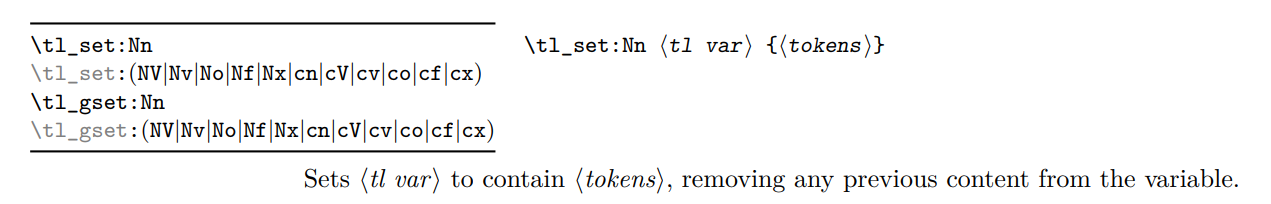
All variants of a function is listed in box on the left. According to the screenshot above, the following functions are provided by ⁵:
```
\tl_set:Nn
\tl_set:NV
\tl_gset:Nx
\tl_gset:cx
```
The syntax of a function is on the top-right.
The detailed description of a function is on the bottom-right.

Scratch variables

Many $LaTeX3$ modules come with predefined “scratch variables” so that users do not have to declare any variable when the code is small. In every chapter, their is a dedicated section to document what scratch variables (as well as constants) are defined.

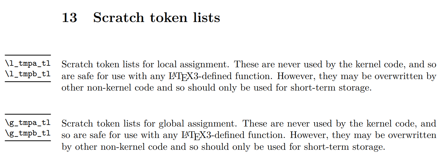
When writing serious $LaTeX3$ code, it is recommended to avoid scratch variables to maximize compatibility.

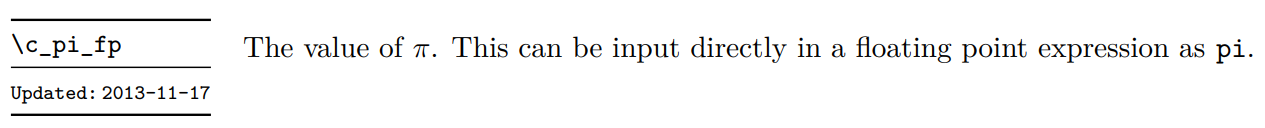
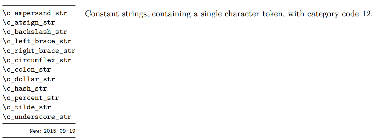
Constants

Some $LaTeX3$ libraries come with pre-defined constants. They will be introduced in a dedicated section.

Summary

$\text{[math]}$ command names must be made up of English letters
$LaTeX3$ command names must be made up of English letters, underline (_) and colon (:)
Use \ExplSyntaxOn and \ExplSyntaxOff to toggle $\text{[math]}$ mode
Special approaches are needed to enter blank space and subscript in $LaTeX3$ mode
Variables and functions follow distinct naming conventions in $LaTeX3$
Detailed information about each argument is encoded in $LaTeX3$ function names
Try to adopt $LaTeX3$ naming convention to increase code readability
Learn to read $LaTeX3$ documentation

Functions & Variables

Defining and using variables

Each module of $LaTeX3$ may use different variable construction format. Therefore, it is important to initialize each variable type with its dedicated function. In general, function ends in new are for declaring new variables; functions that contains set or gset are for modifying variables’ states; functions that contains get are for acquiring variables’ states.

Difference between set and gset

Consider two specific cases \tl_set:Nn and \tl_gset:Nn, which are both used for modifying a token list’s value. What are the differences? As it turns out, the letter g in gset stands for “global”: usually, $\text{[math]}$ only sets the value of a variable locally, i.e. within its own group. That is to say, the modified value will not be visible outside the group. Therefore, if we wish a change to be accessible for all functions, we need to use gset variants.

A concrete example:

\ExplSyntaxOn
\tl_set:Nn \l_tmpa_tl {A}
\group_begin:
\tl_set:Nn \l_tmpa_tl {B}
\par value~inside~group:~\tl_use:N \l_tmpa_tl
\group_end:
\par value~outside~group:~\tl_use:N \l_tmpa_tl

\tl_set:Nn \l_tmpb_tl {A}
\group_begin:
\tl_gset:Nn \l_tmpb_tl {B}
\par value~inside~group:~\tl_use:N \l_tmpb_tl
\group_end:
\par value~outside~group:~\tl_use:N \l_tmpb_tl
\ExplSyntaxOff

The output is:

value inside group: B
value outside group: A
value inside group: B
value outside group: B

It can be seen that \tl_set:Nn only modifies the value inside the group and leaves the value outside untouched; while \tl_gset:Nn changes both values.

In general, the principles of using $LaTeX3$ variables are:

Determine the correct variable type and call the corresponding declaration function (if the number of needed variables is small, conside using scratch variables).
Determine the scope and name the variable according to $LaTeX3$ naming conventions.
Use set or gset functions to modify a variable’s value.
Use corresponding library functions to operate on variables.

Declaring functions (IV-3.2)

In $LaTeX3$ , \cs_set:Npn is usually used for declaring functions. Apart from it, there are also other three functions that serve this job, namely \cs_set_nopar:Npn, \cs_set_protected:Npn and \cs_set_protected_nopar:Npn. Because \cs_set:Npn is used in most cases, we mainly put our focus on it. In fact, their usages are extremely close.

The procedure of declaring a function is as follows:

Determine the number of arguments and their corresponding types ( $\text{[math]}$ macros can accpet at most 9 arguments)
Name the function according to $LaTeX3$ naming convention and define the function with one of functions above.

For example, suppose we are to create a function that concatenates its two arguments with comma. Therefore, we know the number of arguments is 2, and both arguments are of type n. As a result, we can name the function \my_concat:nn. We can define \my_concat:nn like so:

\ExplSyntaxOn
%define \my_concat:nn
\cs_set:Npn \my_concat:nn #1#2 {
    #1,~#2
}
%use \my_concat:nn
\my_concat:nn {a}{b} %result: a, b
\ExplSyntaxOff

Programming interface and user interface

The purpose of $LaTeX3$ is to provide a set of standardized and convenient programming interface to its users. That being said, they are not meant to be easily accessible for everyday $\text{[math]}$ users. In $\text{[math]}$ , many easy-to-use features (e.g. environments, optional arguments) are implemented with sophisticated $\text{[math]}$ tricks. They are a part of the user interface instead of programming interface. Therefore, there is no direct support for them in $LaTeX3$ .

However, $LaTeX3$ can be used to implement robust and handy user interfaces. For example, the xparse package for creating complicated commands and environments is largely implemented with $LaTeX3$ .

Copying the definition of existing functions

Sometimes, it is convenient to copy the definition of existing functions. This can be achieved by invoking \cs_set_eq:NN. In the following example, we create a $LaTeX3$ version of \section function: \my_section:n, and then use it to declare a new “Hello World” section. As we will show later, if a function is declared using $LaTeX3$ naming convention, its macro expansion control will be more convenient.

\ExplSyntaxOn
\cs_set_eq:NN \my_section:n \section
\my_section:n {Hello~World}
\ExplSyntaxOff

Showing the definition of functions

It is possible to show the definition of a function by using \cs_meaning:N. For example, \cs_meaning:N \section gives:

\long macro:->\@startsection {section}{1}{\z@ }{-3.5ex \@plus -1ex \@minus
-.2ex}{2.3ex \@plus .2ex}{\normalfont \Large \bfseries }

Summary

Variables of different types require separate declaration and operation functions.
Generally, functions with new are for creating new variables; functions with set or gset are used to change the state of variables; functions with get are used to acquire the state of variables.
set functions are used to modify variables locally; gset functions are sed to modify variables globally.
In $LaTeX3$ , functions are usually defined with \cs_set:Npn.
Using $LaTeX3$ naming conventions can facilitate macro expansion control.
Use \cs_meaning:N to show the definition of variables.

Macro Expansion Control (V)

Back to the \uppercase example above:

\newcommand{\cmda}{abcd}
\uppercase{abcd\cmda} %ABCDabcd

To show how macro expansion can be resolved with $LaTeX3$ , we first create a $LaTeX3$ equivalent for the function, namely \my_uppercase:n. At this point, the behavior of \my_uppercase:n is the same as \uppercase.

\newcommand{\cmda}{abcd}
\ExplSyntaxOn
\cs_set_eq:NN \my_uppercase:n \uppercase
\my_uppercase:n {abcd\cmda} % ABCDabcd
\ExplSyntaxOff

Now, we discuss two ways to manipulation macro expansion so that the output becomes ABCDABCD (instead of ABCDabcd).

Method 1: change argument specification of functions

At this moment, the argument type of \my_uppercase:n is n, which indicates an unexpanded token list. As a matter of fact, every function has n or N type arguments when first declared. Now, we would like to change to type signature to x, i.e. expanding everything in the token list recursively before being passed to \my_uppercase. In $LaTeX3$ , there is a function dedicated to changing the argument specification of other functions: \cs_generate_variant:Nn. It takes two arguments: the first one is the function we would like to modify; the second one is the new argument specification. Given \my_uppercase:n, we can generate \my_uppercase:x with the help of \cs_generate_variant:Nn and then invoke the new function variant.

\newcommand{\cmda}{abcd}
\ExplSyntaxOn
\cs_set_eq:NN \my_uppercase:n \uppercase
\cs_generate_variant:Nn \my_uppercase:n {x}
\my_uppercase:x {abcd\cmda} % ABCDABCD
\ExplSyntaxOff

Important Notice: \cs_generate_variant:Nn only works for functions following $LaTeX3$ naming convention.

Method 2: use `\exp_args:N` functions (V.4, V.5, V.6)

Declaring new variants with \cs_generate_variant:Nn frequently may be a bit inconvenient. Fortunately, $LaTeX3$ provides a series of \exp_args:N functions that can facilitate macro expansion control when the number of arguments is small.

In short, if we use \cs_generate_variant:Nn to generate and use a new variant function:

\cs_generate_variant:Nn \func:abcd {efgh}
\func:efgh {1}{2}{3}{4}

It will be equivalent to the following \exp_args:N function call:

\exp_args:Nefgh \func:abcd {1}{2}{3}{4}

Using \exp_args:N functions, we can also fully expand the argument for \my_uppercase:n:

\newcommand{\cmda}{abcd}
\ExplSyntaxOn
\cs_set_eq:NN \my_uppercase:n \uppercase
\exp_args:Nx \my_uppercase:n {abcd\cmda} %ABCDABCD
\ExplSyntaxOff

It is worth noticing that \exp_args:N functions can be used to control expansion partially. For example, if a function takes three arguments, and we apply \exp_args:Nc to it, then only the first argument will be modified, while the rest are left untouched. In the example below, we apply c type exansion to the first argument of \NewDocumentCommand from xparse package, which allows us to declare a command named after the content stored in a variable.

% load `xparse` package for this example (will be automatically loaded for newer TeX versions)
\ExplSyntaxOn
% store command name in a variable
\tl_set:Nn \l_tmpa_tl {mycmd}

% use \exp_args:Nc to expand the first arguemnt only
% which allows us to declare a command using the content of \l_tmpa_tl
\exp_args:Nc \NewDocumentCommand{\l_tmpa_tl}{m}{
  \par you~entered~#1
}

% you entered something
\mycmd{something}
\ExplSyntaxOff

Summary

Two ways to control macro expansion in $LaTeX3$ : \cs_generate_variant:Nn and \exp_args:N functions
\cs_generate_variant:Nn only works on functions using $LaTeX3$ naming convention; \exp_args:N series can be applied to arbitrary functions
Since $LaTeX3$ only provides limited number of \exp_args:N functions, one has to fall back to \cs_generate_variant:Nn when the argument combination does not exist.
The arguments of user-defined functions are usually of type n or N. We can leverage the approaches introduced above to modify argument types.
x type expansion may not work in TikZ environments. One can use \edef as an substitution.

LaTeX3: Token List and String

Token list (VII)

Everything that is entered in a tex file can be interpreted as a token. Therefore, token lists are collections of all objects recognized by the $\text{[math]}$ compiler. In $LaTeX3$ , token lists are the most fundamental and frequently used variable type.

Constructing a command in token list

Suppose we would like to call \section*{<title>}, and the <title> is stored in the token list variable \l_tmpa_tl. We can do it as follows:

\ExplSyntaxOn
% put the title in \l_tmpa_tl
\tl_set:Nn \l_tmpa_tl {My~Title}
% construct the command in \l_tmpb_tl
\tl_set:Nx \l_tmpb_tl {\exp_not:N \section* {\l_tmpa_tl}}
\cs_meaning:N \l_tmpb_tl % macro:->\section *{My Title}
% place the content of \l_tmpb_tl into the input stream
\tl_use:N \l_tmpb_tl
\ExplSyntaxOff

In this case, we are using \tl_set:Nx, which means everything inside the curly braces will be expanded completely and recursively. As a result, in the definition of \l_tmpb_tl, the variable name \l_tmpa_tl will be replaced by its value (expanded recursively). Since we do not want to expand the definition of \section, we use \exp_not:N to suppress its expansion.

The x expansion might cause problems when the content of \l_tmpa_tl contains commands. If we only want to put the value of \l_tmpa_tl surrounded by curly braces in \l_tmpb_tl, we can use \exp_not:V in \tl_set:Nx as follows: \tl_set:Nx \l_tmpb_tl {\exp_not:N \section* {\exp_not:V\l_tmpa_tl}}. When being expanded, the \exp_not:V command will place the value of the next variable in the output and prevent the value from being further expanded.

Student management system

Suppose we want to set up an internal student management system in $\text{[math]}$ . We would like to implement the following three commands:

\student: add a new student into the system
\allstudent: show all students, separated by commas
\thestudent: takes one argument and shows the $i$-th student

We will reuse this example many times throughout this tutorial, but with different implementation techniques. Here, we use token list related functions to implement the three commands above.

\documentclass{article}
\usepackage[T1]{fontenc}
\usepackage{expl3}
\usepackage{amsmath, amssymb}

\begin{document}

\ExplSyntaxOn
% stores all students, separated by commas
\tl_new:N \l_student_comma_tl
% stores the name of each student
\tl_new:N \l_student_group_tl
\newcommand{\student}[1]{
    #1% outputs student's name
    % check if \l_student_comma_tl is empty
    % this is a conditional branch statement
    % which we will discuss in the subsequent sections
    \tl_if_empty:NTF \l_student_comma_tl {
        % if empty, do not prepend comma before name
        \tl_put_right:Nn \l_student_comma_tl {#1}
    } {
        % otherwise, prepend comma before name
        \tl_put_right:Nn \l_student_comma_tl {,~#1}
    }
    % put student name in a group and
    % store it in \l_student_group_tl
    \tl_put_right:Nn \l_student_group_tl {{#1}}
}
\newcommand{\allstudent}{
    % outputs \l_student_comma_tl
    \tl_use:N \l_student_comma_tl
}
\newcommand{\thestudent}[1]{
    % outputs the #1-th token in \l_student_group_tl
    \tl_item:Nn \l_student_group_tl {#1}
}
\ExplSyntaxOff

% John and Lisa and David and Emily
\student{John} and \student{Lisa} and \student{David} and \student{Emily}

% John, Lisa, David, Emily
\par\allstudent

% Emily and David and Lisa and John
\par\thestudent{4} and \thestudent{3} and \thestudent{2} and \thestudent{1}

\end{document}

In this solution, we store each name twice in \l_student_comma_tl and \l_student_group_tl. \l_student_comma_tl stores the name of all students, joined by commas, which is used by \allstudent. \l_student_group_tl allows index access for student names, for each student is saved as a group in the token list. Every time one calls \student, the new student name will be inserted into the two token lists.
When inserting into \l_student_comma_tl, there is no need to prepend comma if it is the first name. Therefore, we need to use the conditional statement \tl_if_empty:NTF to specify this behavior.
Notice that we surround the student name with curly braces when inserting into \l_student_group_tl, which effectively encapsulates each student name inside a group. As a result, when calling \tl_item:Nn, the entire group will be returned, which allows us to retrieve the student name as a whole.

String (VIII)

A close relative to token list is string. When we apply \tl_use:N to a token list variable, it is equivalent to typing its content directly in the tex file. If we run the following example

\newcommand{\cmda}{efgh}
\ExplSyntaxOn
\tl_set:Nn \l_tmpa_tl {abcd\cmda}
\tl_use:N \l_tmpa_tl %abcdefgh
\ExplSyntaxOff

then we will get abcdegfh in the document output, because \cmda is stored as a command in \l_tmpa_tl, which is subsequently expanded to efgh. However, If we run the same example with string type, then everything inside the string variable will be interpereted as text instead of command of special character. Consequently, the output in the document becomes abcd\cmda.

\newcommand{\cmda}{efgh}
\ExplSyntaxOn
\str_set:Nn \l_tmpa_str {abcd\cmda}
\str_use:N \l_tmpa_str %abcd\cmda
\ExplSyntaxOff

We can use \tl_to_str:n to convert a token list into a string. It is possible to transform strings back to token lists with \tl_rescan:nn⁶.

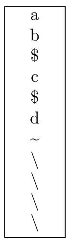
Vertical text node in TikZ

\ExplSyntaxOn
\cs_set:Npn \my_vert_str:n #1 {
  % store argument as string
  \str_set:Nn \l_tmpa_str {#1}
  % traverse the string
  \str_map_inline:Nn \l_tmpa_str {
      % center each character at their own line
      \centering ##1 \par
  }
}
% declare latex interface
\newcommand{\vertstr}[1]{
  \my_vert_str:n {#1}
}
\ExplSyntaxOff

\begin{tikzpicture}
\node[draw=black, text width=1cm] {\vertstr{ab$c$d~\\\\}};
\end{tikzpicture}

Output:

Pitfall of $LaTeX3$ string

$LaTeX3$ ’s string method is implemented with \detokenize. As a result, neither \tl_to_str:n nor \str_set:Nn can guarantee that the string output is exactly the same as users’ input. For example, \detokenize adds an extra space after commands. That is, \verb|abc| becomes \verb |abc|. This can be tricky in some scenarios.

Comparision of token list/string in $LaTeX3$

Very frequently, we need to compare if two token lists or strings are equal. Since the token list library and string library both have their own equality functions, we can choose between \tl_if_eq: (from token list library) and \str_if_eq: (from string library). Unless it is absolutely necessary, it is recommended to use string library’s comparision functions. That is because \tl_if_eq: not only checks if the characters are the same, but it also checks if the category code of each character is the same. As a result, two seemingly identical variables can result in False outcome when using \tl_if_eq:.

LaTeX3: Numeric Evaluation and Boolean Logic

This section mainly consists of code snippets with detailed comments, for the underlying methodology of these topics are similar to other programming languages. Therefore, it is more beneficial to be able to locate the correct APIs in $LaTeX3$ documentation.

Boolean logic (XIII)

\ExplSyntaxOn
% declare new boolean value
\bool_new:N \l_my_bool
% set to true
\bool_set_true:N \l_my_bool
% set to false
\bool_set_false:N \l_my_bool
% boolean based conditional statement
\bool_if:nTF {\l_my_bool} {true} {false} %false
% boolean based while loop
\bool_do_while:nn {\l_my_bool} {}
% boolean based until loop
% boolean functions support C/C++
% style !, || and && operations
\bool_do_until:nn {!\l_my_bool} {}
\ExplSyntaxOff

Integer arithmetic

Implementing modulo operation

It is worth noticing that $LaTeX3$ already has \int_mod:nn. This sample is for demonstration purposes.

\ExplSyntaxOn
\cs_set:Npn \my_mod:nn #1#2 {
  % store #1//#2 in \l_tmpa_int
  \int_set:Nn \l_tmpa_int { \int_div_truncate:nn {#1}{#2} }
  % compute (#1)-\l_tmpa_int*(#2)
  % make sure to surround operands with parentheses
  % so that when #1 is an expression (e.g. 3-2)
  % the order of arithmetic will not change
  \int_eval:n { (#1) - \l_tmpa_int * (#2) }
}
% define LaTeX interface
\newcommand{\mymod}[2]{
  \my_mod:nn {#1} {#2}
}
\ExplSyntaxOff
\mymod{5}{3}\mymod{6}{3}\mymod{7}{1+2}%201

Implementing Caesar cipher

Caesar cipher is a classic substitution cipher in cryptography.

\ExplSyntaxOn
\cs_set:Npn \my_caesar_cipher:n #1 {
  % transform #1 to lower case and store in \l_tmpa_str
  \str_set:Nx \l_tmpa_str {\tl_lower_case:n {#1}}
  % clear \l_tmpb_str to store results
  \str_clear:N \l_tmpb_str
  % \str_map_inline:Nn traverses the string
  % and pass each character as first argument
  \str_map_inline:Nn \l_tmpa_str {
      % `##1 gives the ASCII code of ##1
      % 91 is the ASCII code of 'a'
      % this allows us to compute the offset of ##1
      \int_set:Nn \l_tmpa_int { \int_eval:n {`##1 - 97} }
      % suppose the shifting of our Ceaser cipher is 3
      \int_set:Nn \l_tmpb_int { \int_mod:nn {\l_tmpa_int + 3}{26} }
      % place new character in \l_tmpb_str
      \str_put_right:Nx \l_tmpb_str {
          % this function generates a character given
          % character code and category code
          % because we are dealing with English letters
          % the category code is 11
          \char_generate:nn {\l_tmpb_int + 97}{11}
      }
  }
  % outputs \l_tmpb_str
  \str_use:N \l_tmpb_str
}
\my_caesar_cipher:n {helloworld}%khoorzruog
\ExplSyntaxOff

Integer-based loop and condition

Common integer-based conditional statements:

\int_compare_p: series: compare two integers given a relation and returns a boolean value
\int_compare: series: compare two integers given a relation and execute T code or F code based on the result

Common integer-based loops:

\int_do_while: series
\int_do_until: series
\int_step_function:, \int_step_inline: and \int_step_variable:

1, 2 are often used with \int_incr:N (\int_gincr:N) and \int_decr:N (\int_gdecr:N)

The difference between \int_compare_p:n and \int_compare_p:nNn

One may have noticed that most integer related comparions provide :n and :nNn` variants. They are different in the following ways:

:nNn only supports three types of comparsion: <, > and =
In addition to <, > and ==, :n also supports >=, <= and !=
:n supports chained comparison: a<b<c
The speed of :n is about one fifth of the speed of :nNn

\int_compare_p:nNn {\l_tmpa_int} < {\l_tmpb_int}
% is equivalant to 
\int_compare_p:n {\l_tmpa_int < \l_tmpb_int}

Computing the greatest common divisor (non-recursive)

We implement the Eulidean algorithm to compute the greatest common divisor.

\ExplSyntaxOn
% declare one more scratch variable
\int_new:N \l_tmpc_int
\cs_set:Npn \my_gcd:nn #1#2 {
  % put #1 in \l_tmpa_int
  \int_set:Nn \l_tmpa_int {#1}
  % put #2 in \l_tmpb_int
  \int_set:Nn \l_tmpb_int {#2}
  % loop until \l_tmpb_int equals 0
  \int_do_until:nNnn {\l_tmpb_int} = {0} {
      % update three variables
      \int_set:Nn \l_tmpc_int { \l_tmpb_int }
      \int_set:Nn \l_tmpb_int { \int_mod:nn {\l_tmpa_int}{\l_tmpb_int} }
      \int_set:Nn \l_tmpa_int {\l_tmpc_int}
  }
  % outputs \l_tmpa_int
  \int_use:N \l_tmpa_int
}
\my_gcd:nn {6}{3}~\my_gcd:nn {270}{192}% 3 6
\ExplSyntaxOff

Computing the greatest common divisor (recursive)

As mentioned above, compared to gset functions, set functions only modify variable values within the current group. Using this mechanism, it is possible to imitate a callstack in other programming languages to implement recursive algorithms. In the following example, it is shown that local varialbles will not be modified by subroutines because each set function is guarded by \group_begin: and \group_end:.

\ExplSyntaxOn
\cs_set:Npn \my_gcd_recursive:nn #1#2 {
	\group_begin:
	% all variable assignments will be constrained in this group
	\int_compare:nNnTF {#2} = {0} {
		\int_gset:Nn \g_tmpa_int {#1}
	} {
		\int_set:Nn \l_tmpa_int {\int_mod:nn {#1}{#2}}
		\int_set:Nn \l_tmpb_int {\int_div_truncate:nn {#1}{#2}}
		\exp_args:Nnx \my_gcd_recursive:nn {#2} {\int_use:N \l_tmpa_int}
		% output debug message
		\par $\int_use:N \l_tmpb_int \times #2 + \int_use:N \l_tmpa_int = #1$
	}
	\group_end:
}
\my_gcd_recursive:nn {12546}{156}
\par $\operatorname{gcd}(12546, 156) = \int_use:N \g_tmpa_int$
\ExplSyntaxOff

Output:

× 6 + 0 = 18
× 18 + 6 = 24
× 24 + 18 = 66
× 66 + 24 = 156
× 156 + 66 = 12546
gcd(12546; 156) = 6

Student management system

Now, we implement the aforementioned student management system with integer related functions.

\ExplSyntaxOn
% used to store the name of each student
\tl_new:N \l_student_group_tl
\newcommand{\student}[1]{
  #1% outputs student name
  % put student name in group and then
  % insert into \l_student_group_tl
  \tl_put_right:Nn \l_student_group_tl {{#1}}
}
\newcommand{\allstudent}{
  %\tl_count:N returns the length of a token list
  %\int_step_inline:nn traverses all integers in 
  % the range (1, #1) and pass the loop variable as
  % #1
  \int_step_inline:nn {\tl_count:N \l_student_group_tl}{
      % get the ##1-th element from \l_student_group_tl
      \tl_item:Nn \l_student_group_tl {##1}
      % determine if it is the last element
      % otherwise, append comma
      \int_compare:nNnTF {##1} = {\tl_count:N \l_student_group_tl} {} {,~}
  }
}
\newcommand{\thestudent}[1]{
  % outputs the #1-th item in \l_student_group_tl
  \tl_item:Nn \l_student_group_tl {#1}
}
\ExplSyntaxOff

% John and Lisa and David and Emily
\student{John} and \student{Lisa} and \student{David} and \student{Emily}

% John, Lisa, David, Emily
\par\allstudent

% Emily and David and Lisa and John
\par\thestudent{4} and \thestudent{3} and \thestudent{2} and \thestudent{1}

Three ways to implement nested loop

\ExplSyntaxOn
\par
\int_step_variable:nNn {4} \l_tmpa_tl {
    \int_step_variable:nNn {4} \l_tmpb_tl{
        (\l_tmpa_tl,\l_tmpb_tl)
    }
}
\par
\int_step_inline:nn {4}  {
    \int_step_inline:nn {4}  {
        (#1,##1)
    }
}
\par
\int_set:Nn \l_tmpa_int {1}
\int_do_while:nNnn {\l_tmpa_int} < {5} {
    \int_set:Nn \l_tmpb_int {1}
    \int_do_while:nNnn {\l_tmpb_int} < {5} {
        (\int_use:N \l_tmpa_int,\int_use:N \l_tmpb_int)
        \int_incr:N \l_tmpb_int
    }
    \int_incr:N \l_tmpa_int
}
\ExplSyntaxOff

Output:

(1,1)(1,2)(1,3)(1,4)(2,1)(2,2)(2,3)(2,4)(3,1)(3,2)(3,3)(3,4)(4,1)(4,2)(4,3)(4,4)
(1,1)(1,2)(1,3)(1,4)(2,1)(2,2)(2,3)(2,4)(3,1)(3,2)(3,3)(3,4)(4,1)(4,2)(4,3)(4,4)
(1,1)(1,2)(1,3)(1,4)(2,1)(2,2)(2,3)(2,4)(3,1)(3,2)(3,3)(3,4)(4,1)(4,2)(4,3)(4,4)

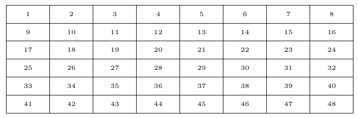
Drawing a square number grid in TikZ

\tikzset{
  mynode/.style={
    minimum height=1cm,
    minimum width=1cm,
    draw,
    anchor=north west
  }
}

\ExplSyntaxOn
\begin{tikzpicture}
\int_step_inline:nn {6} {
  \int_step_inline:nn {8} {
    \node[mynode] at (##1, -#1) {\tiny \int_eval:n {(#1 - 1) * 8 + ##1}};
  }
}
\end{tikzpicture}
\ExplSyntaxOff

Output:

Floating point number (XXIII) and dimension (XX)

The usage of floating point numbers is similar to that of integers: they all have their corresponding new, set, eval and compare functions. It is worth noticing that \fp_eval:n supports a series of scientific functions, which is demonstrated below.

\ExplSyntaxOn
\fp_set:Nn \l_tmpa_fp {2.0}
\par\fp_eval:n {sqrt(\l_tmpa_fp)}% 1.414213562373095
\par\fp_eval:n {sin(\l_tmpa_fp)}% 0.9092974268256817
\par \fp_eval:n {sin(\c_pi_fp)}% 0.0000000000000002384626433832795
\ExplSyntaxOff

It is worth noticing that $LaTeX3$ ’s floating point library is written in pure $\text{[math]}$ , which means it differs from IEEE 754 floating point numbers fundamentally. Nonetheless, after a series of experiments, it is shown that l3fp’s arithmetic accuracy is almost identical to IEEE 754 floating point. The discrapency is neglectable in everyday scenarios ⁷.

Floating points are similar to dimensions, except that dimensions are floating point numbers with a unit (usually in pt). In $LaTeX3$ , dimension variables are represented using IEEE 754 (single precision) floating point internally. Therefore, their processing speed is much faster than l3fp. Dimension variables and floating point variables can be converted from one another using \dim_to_fp:n and \fp_to_dim:n. It is possible to use dimension varialble directly in \fp_eval:n. In this case, dimensions will be converted into pt and lose their unit.

Drawing a rectangular number grid in TikZ

\ExplSyntaxOn
% set width and height of each cell
\dim_new:N \l_w_dim
\dim_set:Nn \l_w_dim {1.2cm}
\dim_new:N \l_h_dim
\dim_set:Nn \l_h_dim {0.5cm}

\tikzset{
  mynode/.style={
    minimum~height=\l_h_dim,
    minimum~width=\l_w_dim,
    draw,
    anchor=north~west
  }
}

\begin{tikzpicture}
\int_step_inline:nn {6} {
  \int_step_inline:nn {8} {
    \node[mynode] at 
    (\fp_eval:n {##1 * \l_w_dim} pt, -\fp_eval:n {#1 * \l_h_dim} pt) 
    {\tiny \int_eval:n {(#1 - 1) * 8 + ##1}};
  }
}
\end{tikzpicture}
\ExplSyntaxOff

Output:

Drawing points on a circle and connect them pairwise

\ExplSyntaxOn
\begin{tikzpicture}
	% draw points on the circle
	\int_step_inline:nn {10} {
		\node[fill=black,
        		circle,
        		inner~sep=0pt,
			outer~sep=0pt,
			minimum~width=1mm] (n#1) at (
			\fp_eval:n {cos(#1 * 36 * \c_one_degree_fp)} cm,
			\fp_eval:n {sin(#1 * 36 * \c_one_degree_fp)} cm
		) {};
	}
	% connect points pairwise
	\int_step_inline:nn {10} {
		\int_step_inline:nn {10} {
			\draw (n#1)--(n##1);
		}
	}
		
	
\end{tikzpicture}
\ExplSyntaxOff

Output:

LaTeX3: Data Structure

Queue (X, XV)

Queues are essential in the implementation of many algorithms. Hence, $LaTeX3$ provides its queue implementation: l3seq.

\ExplSyntaxOn
% create new queue
\seq_new:N \l_my_seq
% empty queue
\seq_clear:N \l_my_seq
% push right into queue
\seq_put_right:Nn \l_my_seq {hello}
\seq_put_right:Nn \l_my_seq {world}
% join elements with '-' and output the result
\seq_use:Nn \l_my_seq {-} % hello-world
% get the length of queue
\seq_count:N \l_my_seq % 2
% pop the rightmost item and store it in \l_tmpa_tl
\seq_pop_right:NN \l_my_seq \l_tmpa_tl
% get the 1st item in the queue
\seq_item:Nn \l_my_seq {1}
% traverse items in queue
% similar functions include \seq_map_inline:
% and \seq_map_function:
\seq_map_inline:Nn \l_my_seq {
    #1
}
\ExplSyntaxOff

We call the l3seq container “queue” or “sequence” instead of “array” or “list”. One of the reasons for this is that index access is read only: one can only access item with \seq_item:Nn, but it is still impossible to modify an item based on index. However, if one wants to create a sequence of integer or floating point numbers, it is possible to take advantage of l3intarray or l3fparray, which allows index-based assignment. As it will be discussed later, they possess some other desirable qualities.

Student management system

\ExplSyntaxOn
% a queue that stores student names
\seq_new:N \l_student_seq
\newcommand{\student}[1]{
  #1% outputs student name
  % push student name to the right
  \seq_put_right:Nn \l_student_seq {#1}
}
\newcommand{\allstudent}{
  % join elements in the queue with comma
  % and then output the result
  \seq_use:Nn \l_student_seq {,~}
}
\newcommand{\thestudent}[1]{
  % outputs the #1-th element in the queue
  \seq_item:Nn \l_student_seq {#1}
}
\ExplSyntaxOff

% John and Lisa and David and Emily
\student{John} and \student{Lisa} and \student{David} and \student{Emily}

% John, Lisa, David, Emily
\par\allstudent

% Emily and David and Lisa and John
\par\thestudent{4} and \thestudent{3} and \thestudent{2} and \thestudent{1}

Bracket matching

\ExplSyntaxOn
\cs_set:Npn \my_paren_match:n #1 {
  % convert #1 into string
  \str_set:Nn \l_tmpa_str {#1}
  % clear working queue
  \seq_clear:N \l_tmpa_seq
  % boolean variable to be set true if parentheses does not match
  \bool_set_false:N \l_tmpa_bool
  \str_map_inline:Nn \l_tmpa_str {
      % \str_case:nn is like the "switch" statement in C
      \str_case:nn {##1} {
          % ------
          % for left brackets, simply push them into the queue
          {(} {
              \seq_put_right:Nn \l_tmpa_seq {(}
          }
          {[} {
              \seq_put_right:Nn \l_tmpa_seq {[}
          }
          % ------
          % ------
          % more work needs to be done for right brackets
          {)} {
              % pop the rightmost element and store it in \l_tmpb_str
              \seq_pop_right:NN \l_tmpa_seq \l_tmpb_str
              % compare it with left round bracket
              % notice that the first argument is passed by value
              \str_if_eq:VnF \l_tmpb_str {(} {
                  % this is executed only when equality does not hold
                  % set "not match" to be true
                  \bool_set_true:N \l_tmpa_bool
                  % exits current loop
                  \str_map_break:
              }
          }
          {]} {
              \seq_pop_right:NN \l_tmpa_seq \l_tmpb_str
              \str_if_eq:VnF \l_tmpb_str {[} {
                  \bool_set_true:N \l_tmpa_bool
                  \str_map_break:
              }
          }
          % ------
      }
  }
  % see if "not match" is true
  \bool_if:NTF \l_tmpa_bool {Not~Match} {
      % see if the working queue is empty
      \seq_if_empty:NTF \l_tmpa_seq {Match} {Not~Match}
  }
}
\par\my_paren_match:n {()()} % Match
\par\my_paren_match:n {([content()])()[]} % Match
\par\my_paren_match:n {([content())()[]} % Not Match
\par\my_paren_match:n {([content()])()[} % Not Match
\ExplSyntaxOff

A very similar data structure is l3clist, which stands for “comma-separated list”. Most functions provided by l3clist is same as l3seq, except that it provides a convenient constructor that allows one to initialize a sequence with comma-separated content. An example is given below.

\ExplSyntaxOn
\clist_new:N \l_my_clist
\clist_set:Nn \l_my_clist {This,is,my,list,1,2,3}
\clist_use:Nn \l_my_clist {-} %This-is-my-list-1-2-3
\ExplSyntaxOff

Dictionary (XVII)

$LaTeX3$ also provides key-value access dictionary container: l3prop. It is similar to dict in Python or map in C++.

\ExplSyntaxOn
% create new dictionary
\prop_new:N \l_my_prop
% clear dictionary
\prop_clear:N \l_my_prop
% add/update key-value pair
\prop_put:Nnn \l_my_prop {key} {val}
% get value given key
\prop_item:Nn \l_my_prop {key} % val
% get number of key-value pairs
\prop_count:N \l_my_prop %1
% traverse key-value pairs
% similar functions include \prop_map_function:
% and \prop_map_tokens:
\prop_map_inline:Nn \l_my_prop {
    (#1, #2)
}
% delete key-value pair
\prop_remove:Nn \l_my_prop {key}
\ExplSyntaxOff

Arabic numerals to English (0-99)

\ExplSyntaxOn

\prop_new:N \l_english_prop
\prop_set_from_keyval:Nn \l_english_prop {
  0=zero,
  1=one,
  2=two,
  3=three,
  4=four,
  5=five,
  6=six,
  7=seven,
  8=eight,
  9=nine,
  10=ten,
  11=eleven,
  12=twelve,
  13=thirteen,
  15=fifteen,
  18=eighteen,
  20=twenty,
  30=thirty,
  40=forty,
  50=fifty,
  80=eighty
}

% extra scratch variable
\tl_new:N \l_tmpc_tl

\cs_set:Npn \my_arabic_to_eng:n #1 {
  \str_set:Nn \l_tmpa_str {#1}
  \prop_if_in:NVTF \l_english_prop \l_tmpa_str {
    % if the number is in the dictionary, output it directly
    % this works for most numbers under 20
    \exp_args:NNV \prop_item:Nn \l_english_prop \l_tmpa_str
  } {
    \int_compare:nNnTF {#1} < {20} {
      % deal with teens
      \exp_args:NNx \prop_item:Nn \l_english_prop {
        \int_eval:n {#1 - 10}
      }
      teen
    } {
      % deal with numbers between 20-99
      % acquire number in tens
      \int_set:Nn \l_tmpa_int {
        \int_div_truncate:nn {#1} {10} * 10
      }
      % acquire number in ones
      \int_set:Nn \l_tmpb_int {
        #1 - \l_tmpa_int
      }
      % #1 = \l_tmpa_int + \l_tmpb_int
      \tl_set:Nx \l_tmpa_tl {\int_use:N \l_tmpa_int}
      
      % outputs the "-ty" word
      \prop_if_in:NVTF \l_english_prop \l_tmpa_tl {
        % no need to construct: get from dict directly
        \exp_args:NNV \prop_item:Nn \l_english_prop \l_tmpa_tl
      } {
        % need to construct the "-ty" word
        \tl_set:Nx \l_tmpc_tl {\tl_head:N \l_tmpa_tl}
        \exp_args:NNV \prop_item:Nn \l_english_prop \l_tmpc_tl
        ty
      }
      % no need to output second digit if it is zero
      \int_compare:nNnF {\l_tmpb_int} = {0} {
        % otherwise, show second digit
        \space
        \tl_set:Nx \l_tmpb_tl {\int_use:N \l_tmpb_int}
        \exp_args:NNV \prop_item:Nn \l_english_prop \l_tmpb_tl
      }
    }
  }
}

\par\my_arabic_to_eng:n {0} % zero
\par\my_arabic_to_eng:n {18} % eighteen
\par\my_arabic_to_eng:n {53} % fifty three
\par\my_arabic_to_eng:n {85} % eighty five

\ExplSyntaxOff

Performance of item-based access

A number of $LaTeX3$ containers provide item-based access methods. For example, \tl_item:Nn, \seq_item:Nn, \prop_item:Nn, etc. Unlike in most programming languages, where the complexity of these methods are constant time (or in some cases, logarithmic time), these methods takes linear time in $LaTeX3$ . That is to say, the larger the container is, the longer the average access time will be.

Fundamentally, $\text{[math]}$ is a text-based macro language. There is no easy way for $\text{[math]}$ scripts to access a computer’s memory space directly. As a result, all containers are essentially constructed with text and requires further interpretation when use. This implies that most $LaTeX3$ containers have extremely high time and memory consumption.

If one wants to store an array of integer or floating point number in $LaTeX3$ , there are two types of high performance containers that allow constant time access, namely l3intarray and l3fparray. In this article, I discussed how to use l3intarray to speed up string reversal.

LaTeX3: Regular Expression (XXVIII)

Regular expression is a powerful tool for pattern matching in text documents. In $LaTeX3$ , the l3regex module provides limited support for standard regular expression syntax. These are some of the frequently used functions in l3regex:

\regex_new:N: creates new regular expression variable
\regex_set:Nn: set the content of a regular expression variable
All of the following functions take either a raw regular expression or regular expression variable as the first argument. Raw regular expressions surrounded by braces requires compilation before use. The \regex_set:Nn function will apply both compilation and storage. Therefore, for a regular exression used multiple times, saving it in a variable may save some time.
\regex_match:nnTF: match a string based on the regular expression and execute T/F code based on the outcome
\regex_count:nnN: count the number of matches and store the result in an integer variable
\regex_extract_once:nnN: extract the first match in the string and store it in a token list variable
\regex_extract_all:nnN: extract all matches in the string and store them in a queue
\regex_split:nnN: split the string based on the regular expression and saved the result in a queue
\regex_replace_once:nnN: replace the first match
\regex_replace_all:nnN:replace all matches

To allow interaction with $\text{[math]}$ , the syntax of l3regex is slightly different from the standard. For more details, please see $LaTeX3$ documentation.

Check if a character is Chinese

\ExplSyntaxOn
% create and compile regex
\regex_new:N \l_chn_regex
% the regular expression for Chinese characters
\regex_set:Nn \l_chn_regex {[\x{3400}-\x{9FBF}]}

\cs_set:Npn \my_is_chn:n #1 {
  % store #1 as string
  \str_set:Nn \l_tmpa_str {#1}
  % clear result queue
  \seq_clear:N \l_tmpa_seq
  % traverse the string
  \str_map_inline:Nn \l_tmpa_str {
      % check if the string matches \l_chn_regex
      \regex_match:NnTF \l_chn_regex {##1} {
          % if so, output Y
          \seq_put_right:Nn \l_tmpa_seq {Y}
      } {
          % otherwise, output N
          \seq_put_right:Nn \l_tmpa_seq {N}
      }
  }
  % show all contents in the queue, separated by white space
  \seq_use:Nn \l_tmpa_seq {\space}
}

% Y N Y N
\par\my_is_chn:n {中a文b}
% N N N N N N N Y Y Y
\par\my_is_chn:n {바탕체ヒラギノ細明體}
\ExplSyntaxOff

Substitute a command with another

In the following example, all occurrence of \cmda is replaced by \cmdb. This example makes use of l3regex’s special syntax.

\newcommand{\cmda}[1]{(#1)}
\newcommand{\cmdb}[1]{[#1]}
\ExplSyntaxOn
\tl_set:Nn \l_tmpa_tl {\cmda{X}~\cmdb{Y}}
\par\tl_use:N \l_tmpa_tl % (X) [Y]
% \c will capture command names
\regex_replace_all:nnN {\c{cmda}} {\c{cmdb}} \l_tmpa_tl
\par \tl_use:N \l_tmpa_tl % [X] [Y]
\ExplSyntaxOff

Generate TikZ picture based on a template

\tikzset{
  mynode/.style={
    outer sep=0pt
  }
}

\ExplSyntaxOn
% this is the template of each node
% which we will fill with regular expressions
\tl_new:N \l_template_tl
\tl_set:Nn \l_template_tl {
  \node[mynode,@1] (@2) at (@3) {@4}; 
}

% counts the total number of nodes
\int_new:N \l_node_counter_int
\int_gset:Nn \l_node_counter_int {0}

% #1: style
% #2: angle
% #3: content
\cs_set:Npn \my_draw_node:nnn #1#2#3 {
  % set our working variable
  \tl_set_eq:NN \l_tmpa_tl \l_template_tl
  % fill style
  \regex_replace_once:nnN {@1} {#1} \l_tmpa_tl
  
  % increment counter
  \int_gincr:N \l_node_counter_int
  % store the name of new node in \l_tmpb_tl
  % node name is generated with \int_to_alph:n
  \tl_set:Nx \l_tmpb_tl {\int_to_alph:n {\l_node_counter_int}}
  % fill node name
  % use \u to replace with the content of a token list
  \regex_replace_once:nnN {@2} {\u{l_tmpb_tl}} \l_tmpa_tl
  
  % calculate the position of the node based on angle
  \tl_set:Nx \l_tmpb_tl {
    \fp_eval:n {3 * cos(#2 * \c_one_degree_fp)}, 
    \fp_eval:n {3 * sin(#2 * \c_one_degree_fp)}
  }
  % fill position
  \regex_replace_once:nnN {@3} {\u{l_tmpb_tl}} \l_tmpa_tl
  
  % fill content
  \regex_replace_once:nnN {@4} {#3} \l_tmpa_tl
  
  % output result
  \tl_use:N \l_tmpa_tl
}

\begin{tikzpicture}
\my_draw_node:nnn {circle,draw}{200}{L}
\my_draw_node:nnn {draw}{160}{A}
\my_draw_node:nnn {circle,draw}{120}{T}
\my_draw_node:nnn {draw}{80}{E}
\my_draw_node:nnn {circle,draw}{40}{X}
\my_draw_node:nnn {draw}{0}{3}

\draw (a)--(b)--(c)--(d)--(e)--(f)--(a);
\end{tikzpicture}

\ExplSyntaxOff

Output:

Processing multi-line text

We can use regular expressions and the xparse package to process multi-line text. In this example, we try to implement a code listing command with line numbering. If we use +v argument specification in \NewDocumentCommand, the argument will be captured as multi-line verbatim. Once the argument is captured as #1, we use \regex_split:nnN {\^^M} {#1} \l_tmpa_seq to split it into multiple lines and save each line in \l_tmpa_seq. The \^^M notation means the carridge return character (ASCII code 13); more details about the ^^ notation can be found in this link.

\ExplSyntaxOn
\NewDocumentCommand{\numberedtext}{+v}{
    \regex_split:nnN {\^^M} {#1} \l_tmpa_seq % split into lines
    \int_set:Nn \l_tmpa_int {1} % line number variable
    \seq_map_inline:Nn \l_tmpa_seq {
        \par
        \group_begin: % we want to limit \ttfamily in this group
        \int_use:N \l_tmpa_int \ttfamily \ % extra space between line number and content
        \tl_to_str:n {##1} % convert content into string
        \group_end:
        \int_incr:N \l_tmpa_int % increment line number counter
    }
}
\ExplSyntaxOff

\numberedtext{\NewDocumentCommand{\numberedtext}{+v}{
    \regex_split:nnN {\^^M} {#1} \l_tmpa_seq
    \int_set:Nn \l_tmpa_int {1}
    \seq_map_inline:Nn \l_tmpa_seq {
        \par
        \group_begin:
        \int_use:N \l_tmpa_int \ttfamily \ 
        \tl_to_str:n {##1}
        \group_end:
        \int_incr:N \l_tmpa_int
    }
}}

Output:

LaTeX3: File I/O (XIX)

In $LaTeX3$ , the APIs of file operations are standardized.

File reading:

\ior_new:N: create new I/O read variable
\ior_open:Nn: open file for reading
\ior_close:N: close file
\ior_get:NN: read one line or a complete group as token list
\ior_str_get:NN: read one line as string
\ior_map_inline:Nn: traverse file as token list
\ior_str_map_inline:Nn: traverse file as string
\ior_if_eof_p:N: check if the tail of a file is reached

File writing:

\iow_new:N: create new I/O write variable
\iow_open:Nn: open file for writing
\iow_close:N: close file
\iow_now:Nn: immediately write content into the file, followed by a line break
\iow_newline:: line break function-this function must be expanded in order to take effect (e.g. \iow_now:Nx \l_tmpa_iow {\iow_newline:}; if the second argument has type n, nothing will happen)

Writing to a file

\ExplSyntaxOn
\iow_open:Nn \g_tmpa_iow {testfile1.txt}
\iow_now:Nx \g_tmpa_iow {hello\iow_newline: world}
\iow_close:N \g_tmpa_iow
\ExplSyntaxOff

The content of testfile1.txt:

hello
world

Reading and parsing comma-separated file

In the following example, we store a series of decimal numbers in a comma-separated file. Then, we read the file and calculate the sum of all numbers.

\ExplSyntaxOn
% write numbers to testfile2.txt
\iow_open:Nn \g_tmpa_iow {testfile2.txt}
\iow_now:Nx \g_tmpa_iow {1.2,2.6,3.7,4.9,5.0,6.5,7.4,8.2,9.4,10.8}
\iow_close:N \g_tmpa_iow

% open file for reading
\ior_open:Nn \g_tmpa_ior {testfile2.txt}
% get the first line
\ior_str_get:NN \g_tmpa_ior \l_tmpa_str
% create function variant
\cs_generate_variant:Nn \regex_split:nnN {nVN}
% split the line into a queue with regular expression
\regex_split:nVN {,} \l_tmpa_str \l_tmpa_seq

% initialize the sum variable
\fp_set:Nn \l_tmpa_fp {0.0}
% traverse the queue
\seq_map_inline:Nn \l_tmpa_seq {
  % sum the numbers
  \fp_add:Nn \l_tmpa_fp {#1}
}

% show result in math mode
$\seq_use:Nn \l_tmpa_seq {+} = \fp_use:N \l_tmpa_fp$
% close file
\ior_close:N \g_tmpa_ior
\ExplSyntaxOff

Output:

1.2+2.6+3.7+4.9+5.0+6.5+7.4+8.2+9.4+10.8=59.7

Memo

Useful techniques:

Many $LaTeX3$ modules provide show functions. They can print the content of variables to the log file, which is very helpful for debug purposes.
$LaTeX3$ also supports generating random numbers or triggering randomized access to token lists or queues.

Because the number of $LaTeX3$ modules is huge, it is very difficult to cover most of them in a limited amount of time. Here, I list some other libraries that are worth looking at:

l3coffins (XXX), l3box (XXIX): allows one to gauge the width/height of objects
l3intarray (XXII), l3fparray (XXIV): high performance numeric arrays
l3sort: sotring queues/token lists
l3msg: generating exception messages

End Note

In this article, I try to breifly introduce the naming convention, the usage of variables and functions and some commonly used modules of $LaTeX3$ . I hope that this organization enables readers to understand the basics of $LaTeX3$ , which allows them to write simple $\text{[math]}$ programs quickly.

There is no doubt that many documents can benefit from the programming capabilities of $LaTeX3$ . It is really pitiful that existing tutorials on $LaTeX3$ is rare, which significantly limits the development of this language. Hopefully, this article can help more people get familar with this powerful tool.

I am not an expert at \expandafter. See more at https://www.zhihu.com/question/26916597/answer/34565213, https://www.tug.org/TUGboat/tb09-1/tb20bechtolsheim.pdf ↩
More about $\text{[math]}$ tokens: https://www.overleaf.com/learn/latex/How_TeX_macros_actually_work:_Part_5 ↩
Turing completeness of $\text{[math]}$ : https://www.overleaf.com/learn/latex/Articles/LaTeX_is_More_Powerful_than_you_Think_-_Computing_the_Fibonacci_Numbers_and_Turing_Completeness ↩
See https://www.overleaf.com/learn/latex/How_TeX_macros_actually_work:_Part_2 ↩
Only a subset of all variants are listed here ↩
Strings are essentially token lists, where each character has category code 11 or 12. What \tl_rescan:nn does is to reassign category code based on provided category code table. Therefore, it is possible to reactivate commands and special characters. See https://tex.stackexchange.com/questions/404108/convert-string-to-token-list. ↩
https://www.alanshawn.com/tech/2020/08/03/l3fp-accuracy.html ↩

Alan Xiang's Blog

LaTeX3: Programming in LaTeX with Ease

Preface

Why LaTeX3?

Handle macro expansion like a boss

Messy interfaces in LaTeX

Goals of LaTeX3

LaTeX3 Naming Conventions (I-1)

Category code and command names

Name of variables

Name of functions

Reading LaTeX3 Documentation

Function documentation

Scratch variables

Constants

Summary

Functions & Variables

Defining and using variables

Declaring functions (IV-3.2)

Copying the definition of existing functions

Showing the definition of functions

Summary

Macro Expansion Control (V)

Method 1: change argument specification of functions

Method 2: use \exp_args:N functions (V.4, V.5, V.6)

Summary

LaTeX3: Token List and String

Token list (VII)

Constructing a command in token list

Student management system

String (VIII)

Vertical text node in TikZ

LaTeX3: Numeric Evaluation and Boolean Logic

Boolean logic (XIII)

Integer arithmetic

Implementing modulo operation

Implementing Caesar cipher

Integer-based loop and condition

Computing the greatest common divisor (non-recursive)

Computing the greatest common divisor (recursive)

Student management system

Three ways to implement nested loop

Drawing a square number grid in TikZ

Floating point number (XXIII) and dimension (XX)

Drawing a rectangular number grid in TikZ

Drawing points on a circle and connect them pairwise

LaTeX3: Data Structure

Queue (X, XV)

Student management system

Bracket matching

Dictionary (XVII)

Arabic numerals to English (0-99)

LaTeX3: Regular Expression (XXVIII)

Check if a character is Chinese

Substitute a command with another

Generate TikZ picture based on a template

Processing multi-line text

LaTeX3: File I/O (XIX)

Writing to a file

Reading and parsing comma-separated file

Memo

End Note

Method 2: use `\exp_args:N` functions (V.4, V.5, V.6)