Scientific Python 3: The Power Of scipy
15 May 2019The scipy package provides a variety of functionalities, which can be applied to a broad range of scientific research. It is quite common for us to ignore that fact that a function already exists in scipy and waste time on finding other packages or reinventing the wheels. In this post, I would show a series of applications for most scipy submodules, just to let readers get a grasp of how versatile this package is. Before the decision of writing one’s own code, it is always better to refer to scipy documentation and see if there is anything helpful.
Numerical integration (scipy.integrate)
Assume that we want to compute the following integration:
\[I = \int^{1/2}_{y = 0}\int^{1-2y}_{x=0} xy~dx~dy\]It can be seen that
\[\begin{align*} I &= \int^{1-2y}_{x=0}x~dx\int^{1/2}_{y = 0}y~dy\\ &= \frac{1}{2} \int^{1/2}_{y = 0}(2y-1)^2y~dy\\ &= \frac{1}{2}\left.\left( y^4 - \frac{4}{3}y^3 + \frac{1}{2}y^2 \right)\right\rvert^{1/2}_{0}\\ &= \frac{1}{96}. \end{align*}\]To compute this with scipy, we can write the following code:
from scipy.integrate import dblquad
intVal, error = dblquad(lambda x, y: x * y, 0.0, 0.5, 0.0, lambda x: 1-2*x)
print(intVal - 1.0/96)
The difference is 1.734723475976807e-18, which indicates that the error is very small.
Convolution (scipy.signal)
Take the gradient Lenna image as an example,
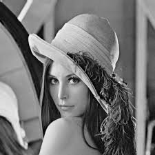
where we would like to apply convolution with a Sobel kernel, which is given by
\[\begin{bmatrix} -1 & 0 & 1\\ -2 & 0 & 2\\ -1 & 0 & 1 \end{bmatrix}.\]With the help of scipy, it can be done with several lines of code:
from PIL import Image
import numpy as np
from scipy.signal import convolve2d
# open image in gradient mode
img = Image.open('2019-05-14-sci-py-1.jpg')
# only take the first channel
# convert to floating point and standardize
npImg = np.asarray(img)[:, :, 0].astype(np.float32) / 255.0
sobel = np.asarray(
[
[-1, 0, 1],
[-2, 0, 2],
[-1, 0, 1]
],
np.float32
)
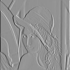
result = convolve2d(sobel, npImg)
# standardize result
result -= result.min()
result /= result.max()
result *= 255.0
pilResult = Image.fromarray(result.astype(np.uint8))
pilResult.save('2019-05-15-sci-py-1.jpg')
The result is shown as below.
Function optimization (scipy.optimization)
Consider the following optimization problem: assume the equation of the circle is \(x^2 + y^2 = 1\), there are two fixed points \(A(0, -1)\) and \(B(1, 0)\) on the circle. Assume that \(P\) is an arbitrary point on the circle. Compute what the coordinate of \(P\) is so that the area of \(\triangle PAB\) is maximized?

The answer is pretty obvious: the area of \(\triangle PAB\) is maximized when \(P\) is farthest away from line \(AB\). The coordinate of \(P\) at this point is \(P\left(-\frac{\sqrt{2}}{2}, \frac{\sqrt{2}}{2} \right)\).
Converting this problem into a constrained optimization problem, denoted point \(P\) by \(P(x, y)\), it is given by:
\[\begin{align*} \max_x f(x) = \frac{1}{2} \cdot \sqrt{2} \cdot \frac{\lvert x - y + 1 \rvert}{\sqrt{2}} = \frac{1}{2} \cdot \lvert x - y + 1 \rvert, \end{align*}\]subject to
\[\begin{gather*} -1 \leq x \leq 1\\ -1 \leq y \leq 1\\ x^2 + y^2 = 1. \end{gather*}\]We can write the following code to solve this problem numerically:
from scipy.optimize import Bounds, NonlinearConstraint, BFGS, minimize

# it is negated because we want to compute the maximum
def target(x):
    return -0.5 * abs(x[0] - x[1] - 1)

def constraintFunc(x):
    return x[0]**2 + x[1]**2

# the bound of x and y
bound = Bounds([-1.0, -1.0], [1.0, 1.0])

constraint = NonlinearConstraint(constraintFunc, 1.0, 1.0)

# using BFGS hessian approximation as an example here
# though it is not ideal for linear functions
res = minimize(target, [0.0, 1.0], method='trust-constr', jac = '2-point', hess = BFGS(), constraints=[constraint], bounds=bound)

print(res)
The result shows:
barrier_parameter: 1.0240000000000006e-08
barrier_tolerance: 1.0240000000000006e-08
         cg_niter: 29
     cg_stop_cond: 1
           constr: [array([1.]), array([-0.70710665,  0.70710691])]
      constr_nfev: [90, 0]
      constr_nhev: [0, 0]
      constr_njev: [0, 0]
   constr_penalty: 1.0
 constr_violation: 1.687538997430238e-14
   execution_time: 0.06944108009338379
              fun: -1.207106781186541
             grad: array([ 0.5, -0.5])
              jac: [array([[-1.4142133 ,  1.41421384]]), array([[1., 0.],
      [0., 1.]])]
  lagrangian_grad: array([7.29464912e-09, 7.29464616e-09])
          message: '`gtol` termination condition is satisfied.'
           method: 'tr_interior_point'
             nfev: 90
             nhev: 0
            niter: 40
             njev: 0
       optimality: 7.29464911613155e-09
           status: 1
        tr_radius: 50837982.540088184
                v: [array([0.35355337]), array([-1.16498790e-07, -5.85727216e-08])]
                x: array([-0.70710665,  0.70710691])
Because \(\frac{\sqrt{2}}{2} \approx 0.707106781\), we can see that the optimizer has given a pretty nice result. In practice, specifying the Jacobian and Hessian matrices for the constraints and the target function is likely to result in faster convergence and better accuracy.
SVD image compression (scipy.linalg)
Suppose that we have a gradient image \(I\), which is an \(m \times n\) matrix. When we apply Singular Value Decomposition (SVD) to it, we have
\[I = USV^T,\]where \(U\) is an \(m \times m\) unitary matrix, \(S\) is an \(m \times n\) rectangular diagonal matrix, and \(V\) is an \(n \times n\) unitary matrix.
We can select the first \(k(k \leq \min(m, n))\) columns of \(U\), the first \(k\) values on the diagonal, the first \(k\) rows of \(V^T\), and it can be seen that these three matrices multiply to a matrix of the same shape of \(I\), because
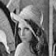
\[(m \times k) \cdot (k \times k) \cdot (k \times n) \rightarrow (m \times n).\]Originally, the image is represented by \(mn\) numbers. Now, we only need \(mk + k + kn = k(m + n + 1)\) numbers. Choosing an appropriate \(k\) can save a lot of storage space. We can write the following program to achieve SVD image compression. The image to be compressed is still Lenna used above.
from PIL import Image
import numpy as np
from scipy.linalg import svd

img = Image.open('2019-05-14-sci-py-1.jpg')
npImg = np.asarray(img)[:, :, 0].astype(np.float32)/255.0

# apply svd
u, s, vt = svd(npImg, compute_uv=True, full_matrices=True)

# how many singular vectors to select
k = 20

print('amount of numbers before compression: ', npImg.size)
# truncate the matrices
newU = u[:, :k]
newS = s[:k]
newVt = vt[:k, :]
print('amount of numbers after compression: ', newU.size + newS.size + newVt.size)

# reconstruct the image
reconImg = np.dot(np.dot(newU, np.diag(newS)), newVt)
reconImg *= 255.0
# clip the reconstructed image
reconImg = np.clip(reconImg, 0.0, 255.0)
pilImage = Image.fromarray(reconImg.astype(np.uint8))

# saving as a lossless format
pilImage.save('2019-05-15-sci-py-3.png')
The output to stdout is:
amount of numbers before compression:  50625
amount of numbers after compression:  9020
And the reconstructed image is shown as below.
Quick Statistics (scipy.stats)
In my opinion, scipy.stats is one of the most powerful scipy submodules. Its functionalities include the p.d.f. and c.d.f. of several dozen probability distributions, parameter estimation, statistical tests, transformations and so on. As an amateur-level statistician, I have never heard of many functions it provides. Not to show my ignorance, I am demonstrating a very simple application of this submodule.
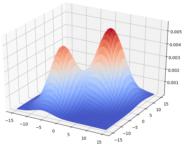
Consider a two-dimensional Gaussian Mixture Model of two classes. Using subscripts to denote the classes, the weight \(w\) and distribution of each class is given by
\[\begin{align*} w_1 &= 0.4\\ \mu_1 &= \begin{bmatrix} -5\\-5 \end{bmatrix}\\ \Sigma_1 &= \begin{bmatrix} 10 & 2\\ 2 & 20 \end{bmatrix}\\ w_2 &= 0.6\\ \mu_2 &= \begin{bmatrix} 5\\5 \end{bmatrix}\\ \Sigma_2 &= \begin{bmatrix} 15 & 3\\ 3 & 20 \end{bmatrix} \end{align*}\]Using \(C_1, C_2\) to denote class 1 and class 2, respectively. It can be seen that
\[\begin{align*} p(C_1 \mid x) &\sim \mathcal{N}(\mu_1, \Sigma_1)\\ p(C_2 \mid x) &\sim \mathcal{N}(\mu_2, \Sigma_2). \end{align*}\]The Gaussian Mixture Model is given by
\[f(x) = w_1p(C_1 \mid x) + w_2p(C_2 \mid x).\]The surface plot of the GMM is shown as below.
By Bayes theorem, we have:
\[\begin{align*} p(x \mid C_1) &= \frac{w_1p(C_1 \mid x)}{w_1p(C_1 \mid x) + w_2p(C_2 \mid x)}\\ p(x \mid C_2) &= \frac{w_2p(C_2 \mid x)}{w_1p(C_1 \mid x) + w_2p(C_2 \mid x)}. \end{align*}\]We would like to explore the shape of the decision boundary of Gaussian Mixture Models. We can do this by selecting a large number of random points, selecting those that are close to the decision boundary, and compute the Pearson’s correlation coefficient of their two components. The program is shown as below (it also includes surface plotting):
from mpl_toolkits.mplot3d import Axes3D
import matplotlib.pyplot as plt
from matplotlib import cm
import numpy as np
from scipy.stats import multivariate_normal, pearsonr

w1, w2 = 0.4, 0.6
mu1 = np.asarray([-5, -5], np.float)
mu2 = np.asarray([5, 5], np.float)
sigma1 = np.asarray([10, 2, 2, 20], np.float).reshape(2, 2)
sigma2 = np.asarray([15, 3, 3, 20], np.float).reshape(2, 2)

dist1 = multivariate_normal(mu1, sigma1)
dist2 = multivariate_normal(mu2, sigma2)

def ComputeGMM(x, y):
    return w1 * dist1.pdf([x, y]) + w2 * dist2.pdf([x, y])

def ProbClass1(x, y):
    return w1 * dist1.pdf([x, y]) / ComputeGMM(x, y)

xs = np.linspace(-15, 15, 40)
ys = np.linspace(-15, 15, 40)
xs, ys = np.meshgrid(xs, ys)
zs = np.vectorize(ComputeGMM)(xs, ys)

# graph the surface of GMM
ax = plt.gca(projection='3d')
ax.plot_surface(xs, ys, zs, cmap = cm.coolwarm)
plt.show()

# a predicate to decide if a sample is close enough
# to the decision boundary
def CloseToBoundary(prob):
    return abs(prob - 0.5) < 0.05

# generate a large number of random points
np.random.seed(0x1a2b3c4d)
# in this case, generate 5000 samples
samples = np.random.uniform(-15.0, 15.0, (5000, 2))
probs = np.vectorize(ProbClass1)(samples[:, 0], samples[:, 1])
closeBool = CloseToBoundary(probs)
print('number of samples close to the decision boundary: ', np.count_nonzero(closeBool))
# extract those samples that are close to the boundary
closeIndices = np.where(closeBool)
closeOnes = samples[closeIndices]

# compute pearson's correlation
print(pearsonr(closeOnes[:, 0], closeOnes[:, 1]))
The result is
number of samples close to the decision boundary:  105
(-0.9925966291080566, 3.9205853694664065e-96)
With a coefficient whose absolute value is very close to one, it is reasonable to speculate that GMM yields a linear decision surface.
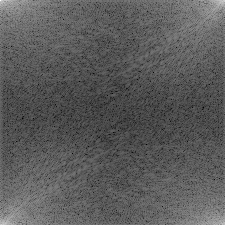
Frequency domain transformations (scipyfft.fftpack)
scipyfft.fftpack provides functions for FFT, DCT and DST. Let’s apply FFT to Lenna and see what the modulus is like.
from PIL import Image
from scipy.fftpack import fft2
import numpy as np

img = Image.open('2019-05-14-sci-py-1.jpg')
npImg = np.asarray(img)[:, :, 0].astype(np.float32)/255.0

# apply fft
freqImg = fft2(npImg)

# compute modulus, apply log to smooth the gradient
modulusImg = np.log(np.abs(freqImg))
modulusImg -= modulusImg.min()
modulusImg /= modulusImg.max()
modulusImg *= 255.0

pilImg = Image.fromarray(modulusImg.astype(np.uint8))
pilImg.save('2019-05-15-sci-py-5.png')
The output is shown below.
Let’s go wild (scipy.spatial, scipy.ndimage)
scipy.spatial submodule is like a mini subset of CGAL, with KD-Tree, triangulation, convex hull and Voronoi diagram algorithm implementations. scipy.ndimage includes a number of image processing routines, such as filtering, morphology, connected component labeling and so on.
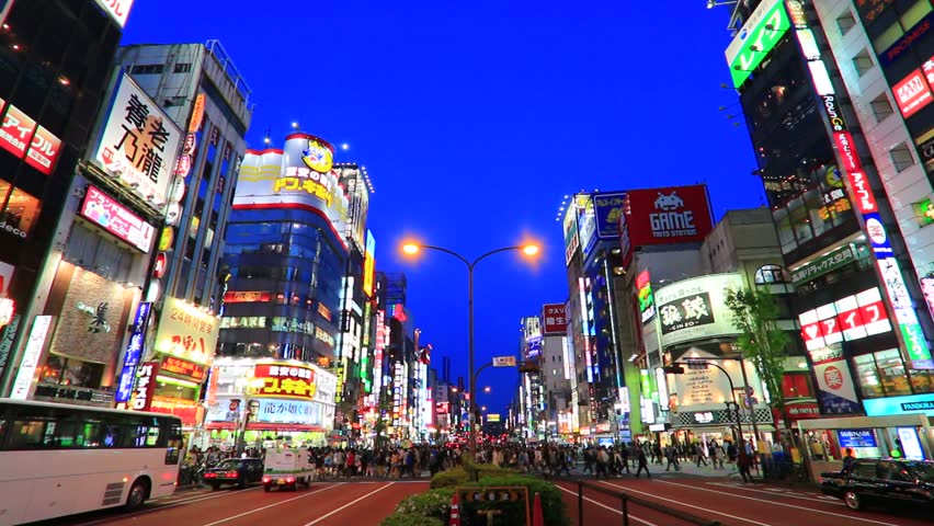
Let’s try to become our own happy little Picasso with all these utilities!
I select the following image as our template.
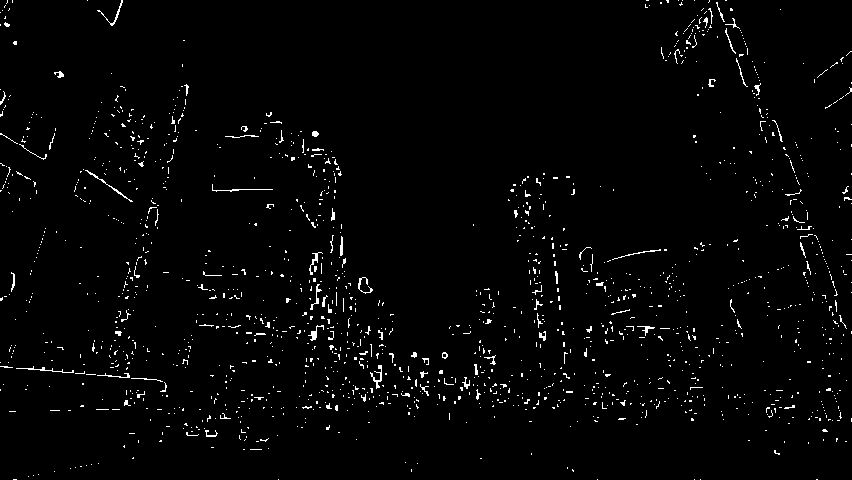
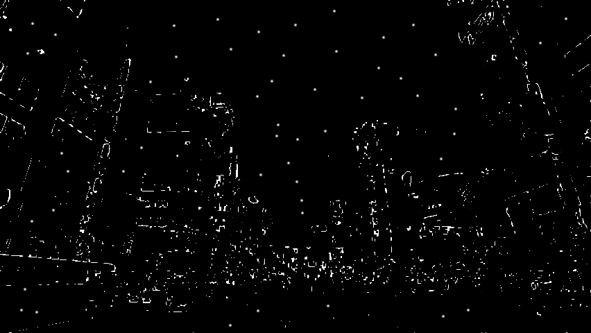
Applying the Sobel operator and some erosion with the following code:
from PIL import Image
from scipy.ndimage import sobel, grey_erosion
import numpy as np

img = Image.open('2019-05-15-sci-py-7.jpg')
npImg = np.asarray(img)[:, :, 0].astype(np.float32)/255.0

# compute sobel operator
sobelX = sobel(npImg, axis = 0)
sobelY = sobel(npImg, axis = 1)
sobelMag = np.sqrt(sobelX **2 + sobelY ** 2)
sobelMag /= sobelMag.max()

# apply thresholding
darkPixels = sobelMag < 0.2
brightPixels = np.logical_not(darkPixels)
sobelMag[darkPixels] = 0.0
sobelMag[brightPixels] = 1.0

# apply a bit of erosion
sobelMag = grey_erosion(sobelMag, size=(3,3))

sobelMag *= 255.0
pilImage = Image.fromarray(sobelMag.astype(np.uint8))
pilImage.save('2019-05-15-sci-py-8.png')
We can acquire this image:
To stylize the image, I used image editing software to paint randomly on the image with black and white brushes. The resulting image is shown as below.
Then, we find out the connected components in the image, and compute their centroids. The next thing to do is to apply triangulation to all centroids, and fill each triangle with the average color taken from the template image. The code is shown as below:
from PIL import Image, ImageDraw
from scipy.ndimage.measurements import label
from scipy.spatial import Delaunay
import numpy as np

img = Image.open('2019-05-15-sci-py-9.png')
npImg = np.asarray(img).astype(np.float32)/255.0

# make the image binary
binImg = npImg > 0.5

# label connected components
labelMat, numLabel = label(img)

def ComputeCentroid(labelId):
    pos = np.where(labelMat == labelId)
    centroid = np.mean(pos, axis=1)
    return centroid

# for each component, find its centroid
centroids = [ComputeCentroid(labelId) for labelId in range(numLabel)]
# eliminate duplicates
centroids = np.unique(centroids, axis = 1)

# apply triangulation to all points
triangles = Delaunay(centroids)

# create a new black image
pilImg = Image.new('RGB', (npImg.shape[1], npImg.shape[0]), (0, 0, 0))
drawer = ImageDraw.Draw(pilImg)

def Revert(p):
    return (p[1], p[0])

# we will extract colors from the template
templateImg = Image.open('2019-05-15-sci-py-7.jpg')
npTemplateImg = np.asarray(templateImg)

# iterate through triangles
for p1, p2, p3 in triangles.simplices:
    # fetch coordinate
    p1, p2, p3 = centroids[p1], centroids[p2], centroids[p3]
    # revert coordinate
    points = list(map(Revert, [p1, p2, p3]))
    # create a temporary pil image
    tempImg = Image.new('1', pilImg.size, 0)
    # draw this triangle in temp image
    tempDraw = ImageDraw.Draw(tempImg)
    tempDraw.polygon(points, fill = 1)
    # convert it into numpy array
    npTempImg = np.asarray(tempImg)
    # using this triangle as the mask to
    # extract pixles from the template image
    pixelData = npTemplateImg[npTempImg]
    # compute average color
    avgColor = np.mean(pixelData, axis = 0).astype(np.uint8)
    # start drawing in the final image
    drawer.polygon(points, fill = tuple(avgColor))


pilImg.save('2019-05-15-sci-py-10.png')
The output is shwon as below:
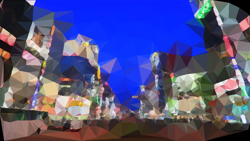
It is amazing how they look alike when being inspected from afar!
Appendix
The code that generates the graph in function optimization
\documentclass[convert=pdf2svg]{standalone}
\usepackage{fourier}
\usepackage{tikz}
\begin{document}
\begin{tikzpicture}
\draw[->, thick] (-1.5, 0) -- (1.5, 0) node[right] {\tiny $x$};
\draw[->, thick] (0, -1.5) -- (0, 1.5) node[above] {\tiny $y$};
\draw (0, -1) -- (1, 0);
\coordinate (itsc) at (-0.9, 0.435889894354067);
\node[yshift=5pt, xshift=-5pt] at (itsc) {$P$};
\node[xshift=5pt, yshift=-5pt] at (0, -1) {$A$};
\node[xshift=5pt, yshift= 5pt] at (1, 0) {$B$};
\draw[fill] (itsc) circle (1pt);
\draw[fill] (0, -1) circle(1pt);
\draw[fill] (1, 0) circle (1pt);
\draw[dashed] (itsc) -- (0, -1);
\draw[dashed] (itsc) -- (1, 0);
\draw (0, 0) circle (1);
\end{tikzpicture}
\end{document}