PyCG 2: Basic 3D Rendering and Lighting

11 Jun 2019

Since it is very common to render 3D objects in practice, this time we are looking at the basics of rendering 3D objects with illumination effects.

Transformation matrices

As it is shown below, there are three matrices that determine how 3D objects are presented on the screen. In order to represnet all three-dimensional transformations with a single matrix, homogeneous coordinates are used. Usually model matrices and view matrices are linear transformations (that is, combinations of translation, rotation and scale), and projection matrices are either orthograpic or perspective.

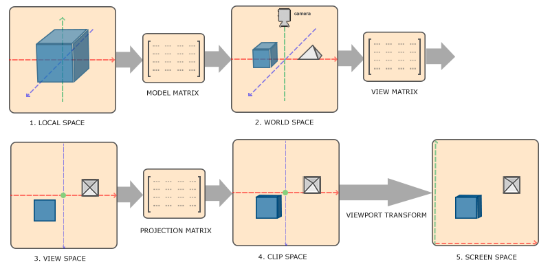
Since transformation matrices are often used, we can write a common library for transformations (which is named as gl_lib/transmat.py in the source folder).

Camera

The figure above shows that the coordinates are transformed from world space to view space based on the camera, which is determined by how the user is trying to view the scene. I choose to implement a simple first-person-shooter-like camera. In this case, there are two parameters controlling the view direction, namely pitch and yaw. These two parameters corresponding to the two degrees of freedom introduced by the mouse. \(\newcommand{\norm}{\operatorname{normalize}}\)

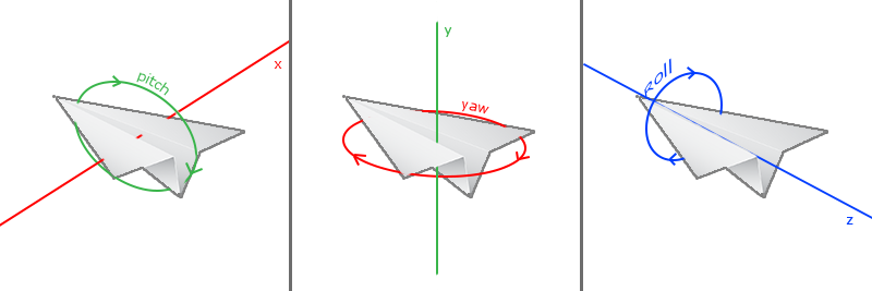
Under this setting, the front (viewing) direction \(\boldsymbol{f}\) is given by

\[\begin{align*} \boldsymbol{f}_x &= \cos(pitch)\cos(yaw),\\ \boldsymbol{f}_y &= \sin(pitch),\\ \boldsymbol{f}_z &= \cos(pitch)\sin(yaw). \end{align*}\]

Since it is conventional to set the default front direction to be towards the negated \(z\) axis, the initial settings would be \(pitch = 0, ~yaw = -\frac{\pi}{2}\). We know that by pressing “a” or “d” in an FPS game, the character would move left or right. In order to do that, we also need to compute the right direction. Because the roll angle does not change, we can always assume that the global up direction is given by the unit \(y\) vector. Therefore, the right direction \(\boldsymbol{r}\) is given by

\[\boldsymbol{r} = \norm\left(\boldsymbol{f} \times (0, 1, 0)^T\right),\]

where \(\times\) denotes cross product. It is also obvious that the up direction \(\boldsymbol{u}\) is given by

\[\boldsymbol{u} = \norm\left(\boldsymbol{r} \times \boldsymbol{f}\right).\]

The implementation the camera can be seen in gl_lib/fps_camera.py.

Shading

Shading refers to depicting depth perception in 3D models or illustrations by varying levels of darkness. One of the shading models that are widely used is Phong shading. Different shading methods can change the style of output image drastically, other shading models include anisotropic shading, toon shading and so on.

In this section, angle brackets \(\langle\rangle\) are used to denote dot product; round dots \(\cdot\) are used to denote scalar-scalar/scalr-matrix product; round circles \(\circ\) are used to denote Hadamard product.

Phong shading

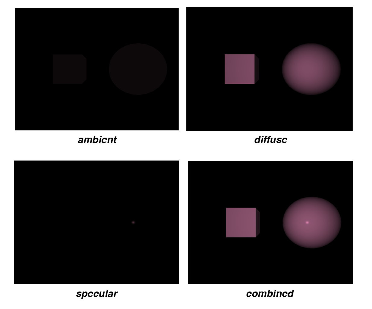
In Phong shading, the final result is the combination of three components: ambient, diffuse and specular. There are several parameters in this model¹:

• \(\boldsymbol{c}_l\): the light color
• \(\boldsymbol{c}_o\): the object color
• \(s_a\): ambient strength
• \(s_s\): specular strength
• \(\boldsymbol{n}\): surface normal vector

• \(\boldsymbol{l}\): light direction vector

  Although the light shines onto objects to make them visible, we always assume that the light direction vector is pointing out from the object surface for the simplicity of calculation. Therefore, if the light source is point light, this vector is given by the normalized difference between the light position and the fragment position. If the light source is directional light, this vector is given by the inverted direction of the light.

• \(\boldsymbol{v}\): view direction vector

  This is given by the normalized difference between the eye position and the fragment position.

• \(\boldsymbol{rf}\): reflection direction vector

  Similar to the convention of light direction vectors, the reflection direction vectors are also point out from the object surface. By the law of reflection, it can be seen that

  \[\boldsymbol{rf} = \norm\left( -\boldsymbol{l} + 2 \cdot \langle\boldsymbol{l}, \boldsymbol{n}\rangle \cdot \boldsymbol{n} \right).\]

• \(p\): specular hightlight effect parameter

  The choice of different \(p\) values results in distinct specular highlight effects. Usually \(p\) is an integer that is greater than 0.

The ambient color \(\boldsymbol{\hat{c}}_a\) is given by

\[\boldsymbol{\hat{c}}_a = s_a \cdot \boldsymbol{c}_l.\]

The diffuse color \(\boldsymbol{\hat{c}}_d\) is given by

\[\boldsymbol{\hat{c}}_d = \max\left(0, \langle\boldsymbol{n}, \boldsymbol{l}\rangle \right) \cdot \boldsymbol{c}_l.\]

The specular color \(\boldsymbol{\hat{c}}_s\) is given by

\[\boldsymbol{\hat{c}}_s = s_s \cdot \left[\max\left(0, \langle \boldsymbol{v}, \boldsymbol{rf} \rangle\right)\right]^{p} \cdot \boldsymbol{c}_l.\]

Finally, the fragment color \(\boldsymbol{\hat{c}}_f\) is given by

\[\boldsymbol{\hat{c}}_f = \left( \boldsymbol{\hat{c}}_a + \boldsymbol{\hat{c}}_d + \boldsymbol{\hat{c}}_s \right) \circ \boldsymbol{c}_o.\]

Anisotropic shading

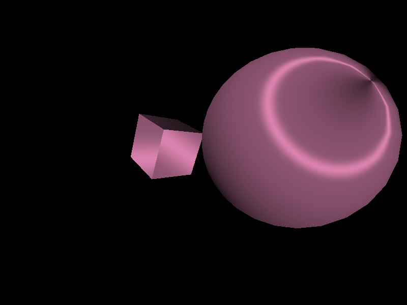
A widely used anisotropic model is the Heidrich–Seidel² anisotropic distribution. Reusing all the notations in Phong shading, Heidrich–Seidel also introduces the following parameters:

• \(\boldsymbol{d}\): thread direction

• \(\boldsymbol{t}\): thread direction based on surface normal

  It is given by

  \[\boldsymbol{t} = \norm\left( \boldsymbol{d} - \langle \boldsymbol{d}, \boldsymbol{n} \rangle \cdot \boldsymbol{n} \right).\]

The diffuse color \(\boldsymbol{\hat{c}}_d\) is given by

\[\boldsymbol{\hat{c}}_d = \sqrt{1 - \langle \boldsymbol{l}, \boldsymbol{t} \rangle^2 } \cdot \boldsymbol{c}_l.\]

The specular color \(\boldsymbol{\hat{c}}_s\) is given by

\[\boldsymbol{\hat{c}}_s = s_s \cdot \left[ \sqrt{1 - \langle \boldsymbol{l}, \boldsymbol{t} \rangle^2}\sqrt{1 - \langle \boldsymbol{v}, \boldsymbol{t} \rangle^2} - \langle \boldsymbol{l}, \boldsymbol{t} \rangle \cdot \langle \boldsymbol{v}, \boldsymbol{t} \rangle \right]^{p} \cdot \boldsymbol{c}_l.\]

The fragment color can be computed in a similar manner.

Putting everything together

The program of this tutorial can be found in the GitHub repository.

Simple introduction:

• Use “wasd” and the mouse to move around the scene
• Press ESC to exit
• Press “o” to toggle anisotropic shading
• Press “p” to take a screenshot