PyCG 4: Spherical Projection

I think most of you may have heard of the concept of dome theaters. Basically, the screen of these type of theaters are not a flat plane, but instead a sphere-like surface.

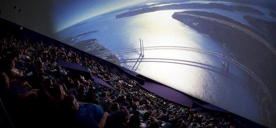
Usually they use special projectors to generate correct images on the screen. But have you ever wondered what it is like if we use a normal projector on one of these screens? With OpenGL and Python, we can develop a simulation program for this scenario very quickly.

How to acquire the image?

A simplified camera/projector model

For simplicity, we are using a very simple mathematical model for the camera and projector in this scenario, which is illustrated as below.

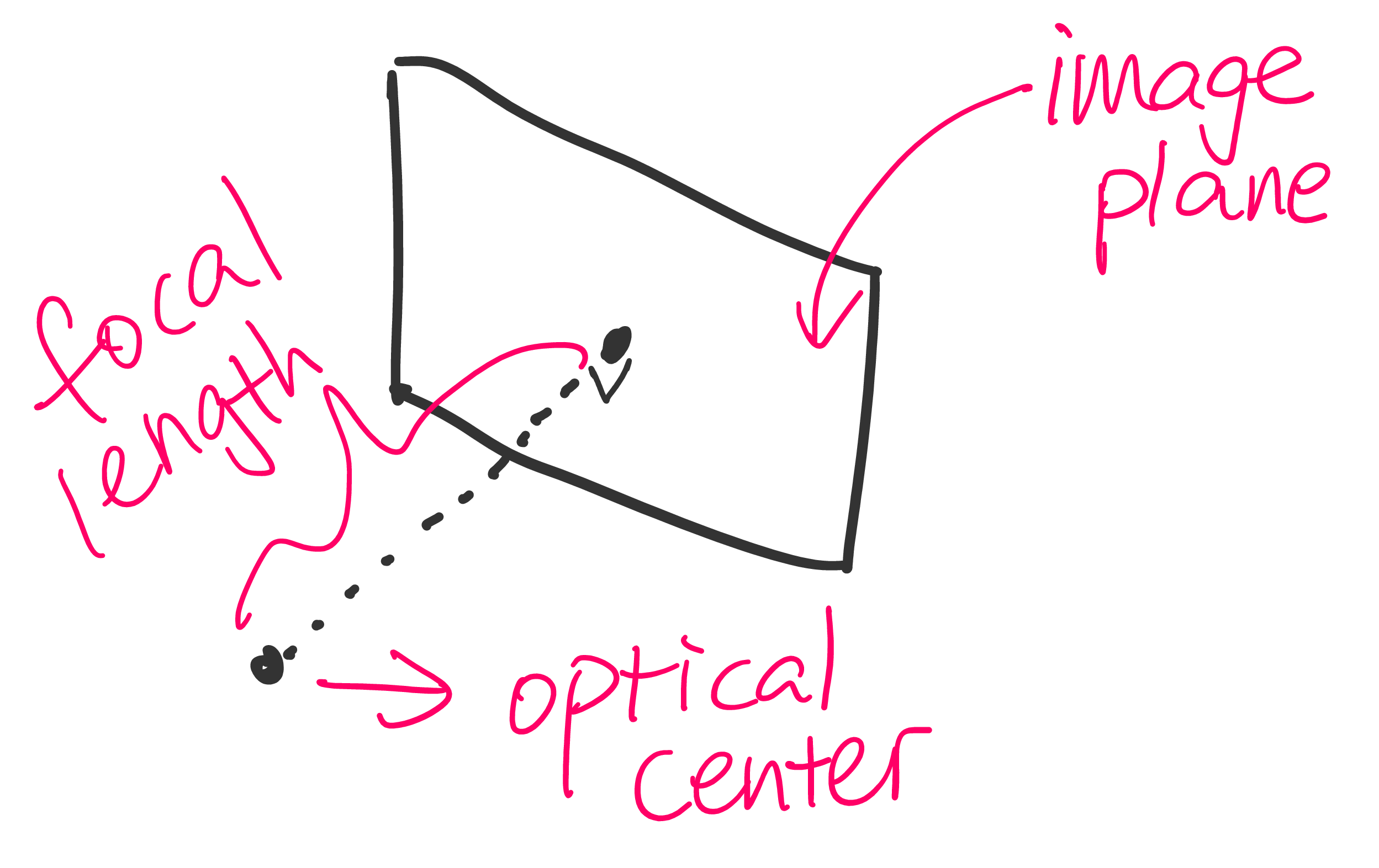
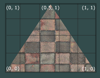
There are two components in this model, namely optical center and image plane. The optical center is right above the center of the image plane, and the distance between optical center and image plane is called focal length. On the image plane, we assume that the coordinate system is identical to the ones of OpenGL textures, which is shown as follows.

Compute the image by ray tracing

Ray tracing is a technique for rendering photo-realistic images. We can compute the projection on the spherical surface by using a modified version of ray tracing. The idea is shown in the following figure.

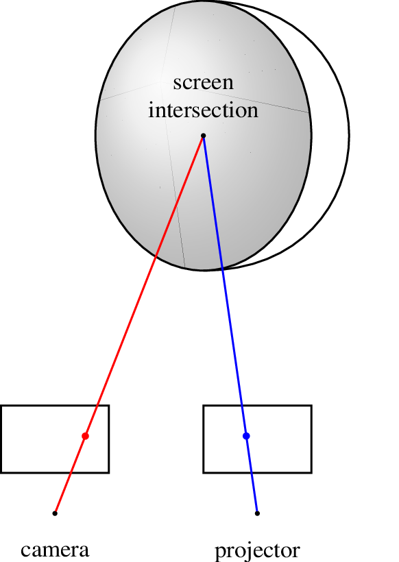
When we look at the screen (which will appear on the camera’s image plane), our sight eventually lands on a point on the sphere (as shown by the red ray). Every point on the sphere may be projected on by some point on the projector’s image plane. In order to find out the corresponding pixel value of a point on the camera’s image plane, we can draw a line (as shown by the blue line) between the screen intersection and projector’s optical center to see if it intersects with projector’s image plane. If so, then the two points will have the same color. More specifically, introduce the following notations:

• \(\bm{o_c}\): the optical center of camera
• \(\bm{o_p}\): the optical center of projector
• \(f_c\): the focal length of the camera
• \(f_p\): the focal length of the projector
• \(\bm{c_c}\): the bottom left corner of camera’s image plane
• \(\bm{x_c}, \bm{y_c}\): the \(x\) and \(y\) axes of the camera’s image plane
• \(\bm{c_p}\): the bottom left corner of projector’s image plane
• \(\bm{x_p}, \bm{y_p}\): the \(x\) and \(y\) axes of the projector’s image plane
• \(\bm{n_c}\): the normalized normal vector of camera’s image plane pointing away from the optical center
• \(\bm{n_p}\): the normalized normal vector of projector’s image plane pointing away from the optical center

Obviously the normal vectors can be computed according to the \(x\) and \(y\) axes. The equation of camera’s image plane is given by

where \(\bm{p_c}\) is an arbitrarily fixed point on the plane. It is reasonable to take \(\bm{p_c} = \bm{o_c} + f_c \bm{n_c}\).

Similarly, the projector’s image plane is given by

where \(\bm{p_p}\) is an arbitrarily fixed point on the plane. We can also take \(\bm{p_p} = \bm{o_p} + f_p \bm{n_p}\). Now for a given 2D location \(\bm{l} = (i, j)^T\) on camera’s image plane (of course, \(i, j \in [0, 1]\)), its 3D coordinates is given by

Therefore the normalized direction \(\bm{d}\) of the red ray in the illustration is given by

Introducing a parameter \(s\), the equation of the red ray is \(\bm{o_c} + s\bm{d}.\) Assume the equation of the sphere surface is given by

where \(z < 0\). Combining it with the ray equation, we have

This is essentially a quadratic equation that is fairly easy to solve. For the solutions, there are three situations, and we only consider the one where the ray intersects with two points on the sphere. For the \(z\) values of those two intersections (denoted by \(z_1, ~z_2\)), there are four possibilities:

1. \(z_1 < 0,~z_2 \geq 0\) or \(z_1 \geq 0,~z_2 < 0\): if the intersection with the hemisphere has \(s \geq 0\), then the screen is visible.
2. \(z_1 < 0, ~z_2 < 0\): the screen is not visible because the sight is blocked by the back side of the screen
3. \(z_2 \geq 0, ~z_2 \geq 0\): the screen is not visible because there is no intersection

Now we only consider the sole intersection with the \(z<0\) hemisphere, which is denoted by \(\bm{v}\). The direction of the blue ray \(\bm{e}\) is given by

Introduce another parameter \(t > 0\), we can write the equation of the blue ray as \(\bm{v} + t\bm{e}\). Combining it with (\(\ref{eqn::proj_plane}\)), we have

which allows us to compute the intersection \(\bm{w}\) between the blue ray and the projector’s image plane. Actually we should do the same intersection detection to make sure that this ray does not intersect with the screen. But for simplicity, we ignore the step here. To retrieve the location of \(\bm{w}\) on the projector’s image plane, which is denoted by \(\bm{l'} = (i', j', k')^T\), we can solve the following equation:

\(\begin{gather} \begin{pmatrix} \vert & \vert & \vert \\ \bm{x_p} & \bm{y_p} & \bm{r} \\ \vert & \vert & \vert \end{pmatrix} \bm{l'} + \bm{c_p} = \bm{w},\\ \bm{l'} = \begin{pmatrix} \vert & \vert & \vert \\ \bm{x_p} & \bm{y_p} & \bm{r} \\ \vert & \vert & \vert \end{pmatrix}^{-1}(\bm{w} - \bm{c_p}), \end{gather}\) where \(\bm{r}\) is an arbitrary vector that is NOT a linear combination of \(\bm{x_p}\) and \(\bm{y_p}\) (for example, \(\bm{x_p} \times \bm{y_p}\)). Because we know that \(\bm{w}\) is on the plane spanned by \(\bm{x_p}\) and \(\bm{y_p}\) only, \(k'\) is guaranteed to be zero, so the choice of \(\bm{r}\) does not matter. Therefore, we can just consider \(\bm{l'} = (i', j')\). If both \(i'\) and \(j'\) are in the range \([0, 1]\), then the color of point \(\bm{l}\) on camera’s image plane will be equal to the color of point \(\bm{l'}\) on projector’s image plane.

Note that this idea can generalize to any type of surfaces, not only spherical ones.

OpenGL implementation

The entire process can be implemented in shaders and therefore be accelarted by GPU hardware. To determine the position of a fragment, the fragment shader will receive a parameter called gl_FragCoord. It is the window coordinates of the fragment. To find the corresponding $\bm{l}$ vector, we can pass in the size of the window as a uniform and compute the quotient.

Demo

The demo can be found in Tutorial_4 folder.

Basic usages:

• Use mouse and “wasd” to look/walk around
• Press Esc to exit
• Press “p” to take screenshots
• Press “o” to switch between controlling camera/projector

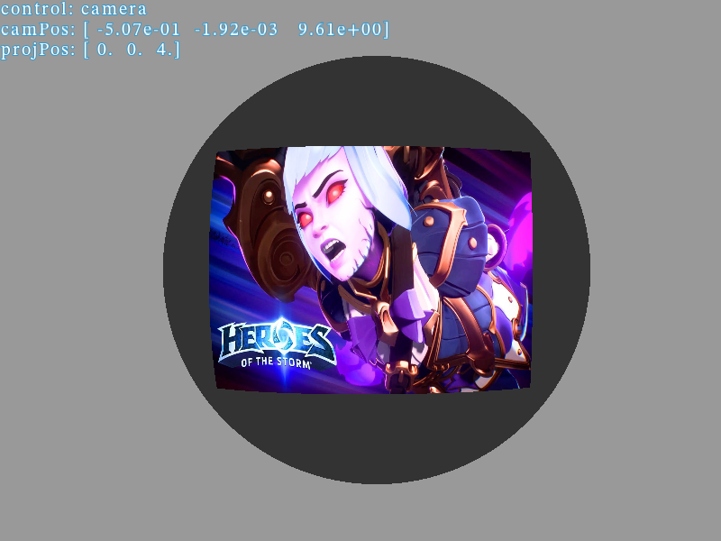
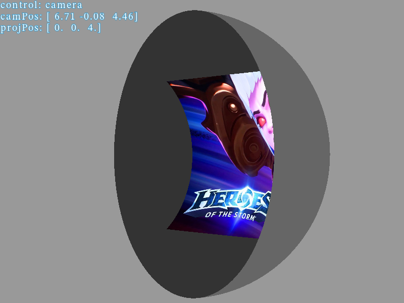
In this article I discuss how to use this demo as an image generator to achieve projection correction.

Appendix

TikZ code for the illustration

\documentclass[convert={density=500}]{standalone}
\usepackage{times}
\usepackage{tikz}
\begin{document}
\begin{tikzpicture}
\tikzstyle{every node}=[font=\tiny, inner sep=0pt, outer sep=0pt]
  \begin{scope}[xscale=0.8]
  \draw (0, 1) to[out=0, in = 0, distance=1.8cm] (0, -1);
  \shade[ball color = gray!40, opacity = 0.4] (0,0) circle (1cm);
  \draw (0,0) circle (1cm);  
  \end{scope}

  % view camera
  \draw[draw=black] (-1.5, -2.5) rectangle ++(0.8, 0.5);
  % projector
  \draw[draw=black] (0, -2.5) rectangle ++(0.8, 0.5);

  \node[yshift=8pt] () at (0, 0) {\parbox{1cm}{\centering{screen\\intersection}}};


  \node[circle, fill=black, minimum size=1pt] (eye) at (-1.1, -2.8) {};
  \draw[red] (eye) -- (0, 0) node[circle, fill=red, minimum size = 1.5pt, pos=0.2] {};

  \node[circle, fill=black, minimum size=1pt] (proj) at (0.4, -2.8) {};
  \draw[blue] (0, 0) -- (proj) node[circle, fill=blue, minimum size = 1.5pt, pos=0.8] {};
  \node[circle, fill=black, minimum size=1pt] at (0, 0) {};

  \node[yshift=-8pt] at (eye) {camera};
  \node[yshift=-8pt] at (proj) {projector};

\end{tikzpicture}
\end{document}