CIS 787: Analytical Data Mining (Fall 2019)
25 Aug 2019Basic Information
- Instructor: Prof. R. Zafarani
- Classroom : Link Hall 105
- Time: Monday, Wednesday 8:00-9:20
- Textbook:
- Introduction to Data Mining [amazon]
- Mining of Massive Datasets [available online]
- Office hours:
- Prof. R. Zafarani: Monday/Wednesday 9:45-10:45 @ CST 4-279
- H. Tian: Tuesday 10:00-12:00 @ CST 0-124
Data
Terminologies
- A dataset is a collection of data objects and their attributes.
- An attribute is a property or characteristic of an object. It is different from attribute value, which is the number/symbol assigned to that attribute.
- Aliases of attributes: variable, dimension, field, characteristic, feature…
- A collection of attributes describe an object.
- Aliases of data obects: record, data point, observation, event, point, case, sample, entity, instance…
- Attribute types (by transformations allowed)
- Nominal (supports identifying distinctness, i.e. \(=\) and \(\neq\))
- Ordinal (also supports identifying order, i.e. \(<, \leq, >\) and \(\geq\))
- Interval (also supports addition, i.e. \(+\) and \(-\))
- Ratio (also supports multiplication, i.e. \(\times\) and \(\div\))
The difference between Ordinal and IntervalThe most important characteristic of Interval attributes is that they support addition and subtraction. That is, their sum and difference make sense. For example, cloth sizes (M, L, XL) is ordinal, as they support comparison, but one cannot apply addition or difference to them. Time in terms of AM or PM is interval, as you can subtract two time points to get the duration.
The types with larger index value will inherit all valid operations of the smaller ones, as well as allowing more operations on their own. Nominal and ordinal attributes are called qualitative attributes; interval and ratio attributes are called quantitative attributes.
- Attribute types (by number of values)
Data processing methods
-
Aggregation: combining two or more objects into a single object. This approach can reduce the dataset size; provide a high-level view on the dataset; cancel some noise within the dataset.
-
Sampling: selecting a subset of data objects to be analyzed. Approaches: sampling with replacement, sampling without replacement, stratified sampling. Stratified sampling guarantees that the distribution of groups after sampling is identical to that of original dataset’s.
Dimensionality reduction
- Curse of dimensionality: many types of data analysis become significantly harder as the dimensionality of the data increases. Specifically, as dimensionality increases, the data becomes increasingly sparse [wiki].
When dimensionality increases, the data points because increasingly sparse in the sample space. As a result, all the samples in the dataset tend to concentrate in a small region of the sample space, making them closer to each other. For example, we can generate \(n\) random vectors of \(d\) dimensions, where each element ranges in \([0, 100]\). Then, we compute their pairwise distances, and let
\[\gamma = \log\left(\frac{\mbox{maimum pairwise distance} - \mbox{minimum pairwise distance}}{\mbox{minimum pairwise distance}}\right).\]The surface plot of \(\gamma\) is shown as below.
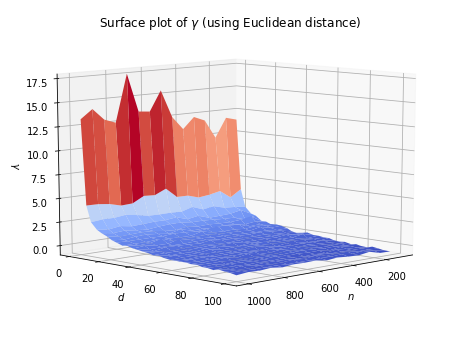
It can be seen that as \(n\) increases, the value of \(\gamma\) increases slightly. But its effect is insignificant compared to the dominant impact brought by the increment of \(d\). Overall, \(\gamma\) tends to be very close to 0 when dimensionality increases. Therefore, one needs to be very careful when computing distance/similarity in high dimensional space, as the distance between samples are closer.
Principle Component Analysis (PCA)
Suppose there are \(m\) data instances each with \(n\) features. Denote the \(i\)th feature of \(j\)th instance by \(x^{(j)}_i\). The \(j\)th instance can therefore be written as
\[\bm{x}^{(j)} = \left\{x^{(j)}_1, x^{(j)}_2, \ldots, x^{(j)}_n \right\}^T.\]For convenience, we can represent all data with a data matrix \(\bm{X} \in \mathbb{R}^{m\times n}\), where
\[\begin{align*} \bm{X} = \begin{bmatrix} x^{(1)}_1 & x^{(1)}_2 & \cdots & x^{(1)}_n\\ x^{(2)}_1 & x^{(2)}_2 & \cdots & x^{(2)}_n\\ \vdots & \vdots & \ddots & \vdots\\ x^{(m)}_1 & x^{(m)}_2 & \cdots & x^{(m)}_n \end{bmatrix} = \begin{bmatrix} \bm{x}^{(1)^{T}}\\ \bm{x}^{(2)^{T}}\\ \vdots \\ \bm{x}^{(m)^{T}} \end{bmatrix}. \end{align*}\]We can also view the data matrix by column, where \(i\)th column \(\bm{a}^{(i)} \in \mathbb{R}^m\) is all values of \(i\)th attribute.
\[\begin{align*} \bm{X} = \begin{bmatrix} x^{(1)}_1 & x^{(1)}_2 & \cdots & x^{(1)}_n\\ x^{(2)}_1 & x^{(2)}_2 & \cdots & x^{(2)}_n\\ \vdots & \vdots & \ddots & \vdots\\ x^{(m)}_1 & x^{(m)}_2 & \cdots & x^{(m)}_n \end{bmatrix} = \begin{bmatrix} \bm{a}^{(1)}, \bm{a}^{(2)}, \cdots, \bm{a}^{(n)} \end{bmatrix}. \end{align*}\] \[\newcommand{\cov}{\operatorname{cov}}\]The idea of PCA is to eliminate covariace among different attributes so that each attribute can be more descriptive. What PCA does is to find a projection matrix to place the dataset under a new base, where the (linear) dependency among attributes are canceled after the transformation.
The dependency is measured by covariance. Given two \(m\) dimensional vector \(\bm{x}\) and \(\bm{y}\), the covariance between them writes
\[\begin{align*} \cov\left(\bm{x}, \bm{y}\right) &= \frac{1}{m-1} \sum_{i = 1}^{m} (\bm{x}_i - \bar{\bm{x}})(\bm{y}_i - \bar{\bm{y}})\\ &= \frac{1}{m-1} \left\langle \bm{x} - \bar{\bm{x}}, \bm{y} - \bar{\bm{y}} \right\rangle \end{align*},\]where \(\bar{\cdot}\) denotes the mean value of the vector, \(\langle \cdot\rangle\) denotes inner product, and the subscript denotes the \(i\)th element.
Define the centered data matrix \(\bar{\bm{X}}\) to be
\[\begin{align} \bar{\bm{X}} &= \begin{bmatrix} \bm{a}^{(1)} - \bar{\bm{a}^{(1)}}, \bm{a}^{(2)} - \bar{\bm{a}^{(2)}}, \cdots, \bm{a}^{(n)} - \bar{\bm{a}^{(n)}} \end{bmatrix}\nonumber\\ &= \begin{bmatrix} x^{(1)}_1 -\frac{1}{m}\sum_{i=1}^{m}x^{(i)}_1 & x^{(1)}_2 - \frac{1}{m}\sum_{i=1}^{m}x^{(i)}_2 & \cdots & x^{(1)}_n - \frac{1}{m}\sum_{i=1}^{m}x^{(i)}_n \\ x^{(2)}_1 -\frac{1}{m}\sum_{i=1}^{m}x^{(i)}_1 & x^{(2)}_2 - \frac{1}{m}\sum_{i=1}^{m}x^{(i)}_2 & \cdots & x^{(2)}_n- \frac{1}{m}\sum_{i=1}^{m}x^{(i)}_n \\ \vdots & \vdots & \ddots & \vdots\\ x^{(m)}_1 -\frac{1}{m}\sum_{i=1}^{m}x^{(i)}_1 & x^{(m)}_2 - \frac{1}{m}\sum_{i=1}^{m}x^{(i)}_2 & \cdots & x^{(m)}_n - \frac{1}{m}\sum_{i=1}^{m}x^{(i)}_n \end{bmatrix}\label{eqn::centered_data}. \end{align}\]That is, \(\bar{\bm{X}}\) is the matrix where each attribute is subtracted by its average value. In fact, the computation in \((\ref{eqn::centered_data})\) can be expressed in terms of matrix multiplication, with the help of centering matrix. The \(m\) dimensional centering matrix \(\bm{M}_m\) is given by
\[\bm{M}_m = \bm{I}_m - \frac{1}{m}\bm{1}\bm{1}^T.\]With this in hand, we can write \(\bar{\bm{X}} = \bm{M}_m\bm{X}\) (this is fairly easy to prove with \((\ref{eqn::centered_data})\)). Consider the following matrix
\[\begin{align*} \bar{\bm{X}}^T\bar{\bm{X}} &= \begin{bmatrix} \left(\bm{a}^{(1)} - \bar{\bm{a}^{(1)}}\right)^T\\ \left(\bm{a}^{(2)} - \bar{\bm{a}^{(2)}}\right)^T\\ \vdots\\ \left(\bm{a}^{(n)} - \bar{\bm{a}^{(n)}}\right)^T \end{bmatrix} \begin{bmatrix} \bm{a}^{(1)} - \bar{\bm{a}^{(1)}}, \bm{a}^{(2)} - \bar{\bm{a}^{(2)}}, \cdots, \bm{a}^{(n)} - \bar{\bm{a}^{(n)}} \end{bmatrix}\\ &= \begin{bmatrix} \langle \bm{a}^{(1)} - \bar{\bm{a}^{(1)}}, \bm{a}^{(1)} - \bar{\bm{a}^{(1)}}\rangle & \langle \bm{a}^{(1)} - \bar{\bm{a}^{(1)}}, \bm{a}^{(2)} - \bar{\bm{a}^{(2)}}\rangle & \cdots & \langle \bm{a}^{(1)} - \bar{\bm{a}^{(1)}}, \bm{a}^{(n)} - \bar{\bm{a}^{(n)}}\rangle\\ \langle \bm{a}^{(2)} - \bar{\bm{a}^{(2)}}, \bm{a}^{(1)} - \bar{\bm{a}^{(1)}}\rangle & \langle \bm{a}^{(2)} - \bar{\bm{a}^{(2)}}, \bm{a}^{(2)} - \bar{\bm{a}^{(2)}}\rangle & \cdots & \langle \bm{a}^{(2)} - \bar{\bm{a}^{(2)}}, \bm{a}^{(n)} - \bar{\bm{a}^{(n)}}\rangle\\ \vdots & \vdots & \ddots & \vdots\\ \langle \bm{a}^{(n)} - \bar{\bm{a}^{(n)}}, \bm{a}^{(1)} - \bar{\bm{a}^{(1)}}\rangle & \langle \bm{a}^{(n)} - \bar{\bm{a}^{(n)}}, \bm{a}^{(2)} - \bar{\bm{a}^{(2)}}\rangle & \cdots & \langle \bm{a}^{(n)} - \bar{\bm{a}^{(n)}}, \bm{a}^{(n)} - \bar{\bm{a}^{(n)}}\rangle \end{bmatrix}. \end{align*}\]It can be seen that \(\bm{C} = \frac{1}{n-1}\bar{\bm{X}}^T\bar{\bm{X}}\) is exactly the covariance matrix of all attributes. On the diagonal, it is the variance of each attribute. In order to eliminate dependency among different attributes (i.e. the covariance), we would like the non-diagonal elements in \(\bm{C}\) to be zero.
Because \(\bm{C}\) is symmetric, we can apply eigendecomposition to it, so that
\[\begin{align}\label{eqn::eigen_decomp_c} \bm{C} = \bm{U}\bm{\Lambda}\bm{U}^{T}, \end{align}\]where each column of \(\bm{U}\) stores \(\bm{C}\)’s eigenvectors, and each diagonal element of diagonal matrix \(\bm{\Lambda}\) is \(\bm{C}\)’s eigenvalue. Notice that \((\ref{eqn::eigen_decomp_c})\) is only true for symmetric matrices, beacuse \(\bm{U}\) is an orthogonal matrix so that \(\bm{U}^{-1}=\bm{U}^T\).
Now we would like to apply some projection \(\bm{P}\) to the rows of \(\bar{\bm{X}}\), so that the covariace after it is canceled. Consider the covariance matrix after transformation, that is
\[\begin{align*} \frac{1}{n-1}(\bar{\bm{X}}\bm{P})^T(\bar{\bm{X}}\bm{P}) &= \frac{1}{n-1}\bm{P}^T\bar{\bm{X}}^T\bar{\bm{X}}\bm{P}\\ &= \bm{P}^T\bm{C}\bm{P}\\ &= \bm{P}^T \bm{U}\bm{\Lambda}\bm{U}^{T} \bm{P}. \end{align*}\]By orthogonality, it is easy to see that if we let \(\bm{P} = \bm{U}\), then the new covariance matrix after projection would be equal to \(\bm{\Lambda}\), which is a diagonal matrix. Now, the covariance is eliminated, leaving only variance terms in the covariance matrix.
Applications of PCA
-
Decorrelate attributes
To decorrelate the attributes, simply right multiply the centered data matrix with \(\bm{U}\), that is, \(\bar{\bm{X}}\bm{U}\).
-
Dimensionality reduction
Since the covariance matrix after transformation is \(\bm{\Lambda}\), it can be seen that the variance of attributes after transformation is the eigenvalues of \(\bm{C}\). It is easy to see that \(\bm{C}\) is a positive semi-definite matrix, so its eigenvalues are non-negative [properties of eigenvalues] [definiteness of a matrix]. Usually the matrix \(\bm{U}\) and \(\bm{\Lambda}\) are arranged such that the eigenvalues are in decreasing order along \(\bm{\Lambda}\)’s diagonal. To reduce dimensionality, we can select the first \(k\) columns of \(\bm{U}\) (denoted by \(\bm{U}_k\)), and represent the data with \(\bar{\bm{X}}\bm{U}_k\).
On selecting the value of \(k\):
- One can select based on the eigenvalue (i.e. the variance of an attribute after transformation). We can select \(k\) such that the eigenvalues after \(k\) are reasonably small. That is, they are not very descriptive.
- Energy-based selection: One can sum up all the eigenvalues, and select top-\(k\) eigenvectors until their corresponding eigenvalues exceed a certain threshold (e.g. 90% of the sum of all eigenvalues).
-
Noise cancellation
To cancel noise in the data, we can apply dimensionality reduction first, and then use a inverse transformation to map the data back to their original dimensionality. That is, compute \(\left(\bar{\bm{X}}\bm{U}_k\right)\bm{U}^T_k\). By doing so, the attributes with low variance are eliminated, resulting in purer data. A similar example can be seen in the video in this post (though the purpose here is for compression).
Classification
In machine learning and statistics, classification is the problem of identifying to which of a set of categories (sub-populations) a new observation belongs, on the basis of a training set of data containing observations (or instances) whose category membership is known [wiki].
Decision trees
In computer science, Decision tree learning uses a decision tree (as a predictive model) to go from observations about an item (represented in the branches) to conclusions about the item’s target value (represented in the leaves). It is one of the predictive modeling approaches used in statistics, data mining and machine learning. Tree models where the target variable can take a discrete set of values are called classification trees; in these tree structures, leaves represent class labels and branches represent conjunctions of features that lead to those class labels [wiki].

Hunt’s algorithm
The Hunt’s algorithm is one of the earliest methods to build decision trees. Its pseudocode can be seen as below.
How to split a node?
Usually, we split on a particular attribute on a node. If the attribute is discrete, we can split the node based on values, or based on a group of values. If the attribute is continuous, we can split the range of value into several bins.
How to find the best split?
We can use an attribute test to measure the effectiveness of a split. The idea is that the distribution of data after splitting should be as skewed as possible, because a uniform distribution of data after splitting does not help classifying much. Therefore, we introduce the concept of impurity – the data should be as “impure” as possible after the split.
Denote the fraction of records belong to class \(i\) at node \(t\) by \(p_t(i)\), \(i \in \{1, 2, \ldots, n\}\). There are three different measures of impurity, which are listed as follows. The best scenario is when every sample of a node belongs to one class; the worst scenario is when the class label is uniformly distributed.
-
Entropy (assume \(p_t(i) \log_2 p_t(i) = 0\) when \(p_t(i) = 0\))
\[\begin{align*} \mbox{Entropy}(t) = -\sum_{i = 1}^{n} p_t(i) \log_2 p_t(i) \end{align*}\]- Best: 0
- Worst: \(\log_2 n\).
-
\[\begin{align*}
\mbox{Gini}(t) = 1 - \sum_{i = 1}^{n} p^2_t(i)
\end{align*}\]
- Best: 0
- Worst: \(\frac{n-1}{n}\)
-
Classification error
\[CE(t) = 1 - \max_i \left[ p_t(i) \right]\]- Best: 0
- Worst: \(\frac{n-1}{n}\)
The best split is decided based on the gain of split. Assume that a split instance divides the parent node into $k$ child nodes \(v_1, v_2, \ldots, v_k\). The gain of the split is given by
\[\Delta = I(\mbox{parent}) - \sum_{j = 1}^{k} \frac{N(v_j)}{N(\mbox{parent})}I(v_j),\]where \(I(\cdot)\) denotes the impurity measure and \(N(\cdot)\) denote the number of records at each node. The best split is the split with maximum gain. When the impurity measure is entropy, the gain is also known as information gain (denoted by \(\Delta_{\mbox{info}}\)).
However, information gain/Gini gain tend to favor small and fragmented splits, which may lead to bad generalization. Therefore, another splitting criterion that penalizes the number of splits is introduced, which is called gain ratio. More concretely,
\[\mbox{Gain ratio} = \frac{\Delta_{\mbox{info}}}{\mbox{SplitINFO}},\]where
\[\mbox{SplitINFO} = -\sum_{j = 1}^{k} \frac{N(v_j)}{N(\mbox{parent})} \log \frac{N(v_j)}{N(\mbox{parent})}.\]It can be seen that if an attribute produces a large number of splits, it will have a greater \(\mbox{SplitINFO}\), which eventually reduces its gain ratio.
Underfitting and Overfitting
In supervised learning, underfitting happens when a model unable to capture the underlying pattern of the data. Meanwhile, Overfitting happens when our model captures the noise along with the underlying pattern in data. Underfitting and overfitting are essentially two extremes of bias-variance tradeoff, which can be illustrated by the bulls-eye diagram below. Suppose the center of the target is a model that perfectly predicts correct values, and the predictions of the model is denoted by “\(\times\)”.
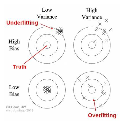
In the case of underfitting, the overall mass of predictions is far away from truth, which means the machine learning algorithm fails to learn the underlying patterns of the data. In the case of overfitting, the overall mass of prediction is somehow close to the center of the diagram, but individual predictions are noisy and far from the truth. In we introduce a test set, when underfitting happens, both the training error and testing error are high. When overfitting happens, the training error is low, but the testing error is high.
Possible cause of underfitting: the machine learning model is too simple for the dataset.
Possible cause of overfitting:
- Noisy data
- Insufficient (representing) examples
- Excessive model complexity
Dealing with overfitting
- Occam’s razor: Given two models with the same generalization errors, the simpler model is preferred over the more complex model.
- Pre-pruning: the tree-growing algorithm is halted before generating a fully grown tree that fits the entire training data. To do this, a more restrictive stopping condition is used. However, it is very difficult to select the threshold for early termination. Too high of a threshold will result in underfitting, where as too low of a threshold may not be enough to counter overfitting.
- Post-pruning: At first, the decision tree is grown to its maximum size, which is following by a pruning step. The fully-grown tree is trimmed in a bottom-up fashion, where a subtree can either be replaced by a node or the mostly selected brach of that subtree. Post-pruning tends to give better results than pre-pruning, because it works on a fully-grown tree. However, it is computationally expensive.
Minimum Description Length (MDL): Comparing effectiveness of decision trees
Given two different decision trees, we can compare their overall effectiveness based on a heuristic called Minimum Description Length (MDL). With MDL, the total description length of a tree is given by
\[\mbox{Cost}(tree, data) = \mbox{Cost}(tree) + \mbox{Cost}(data \mid tree).\]- \(\mbox{Cost}(tree)\) is the cost of encoding all the nodes in the tree. Each internal node of the tree is encoded by the ID of the splitting attribute, If there are \(m\) attributes, the cost of encoding each attribute is \(\lceil\log_2 m \rceil\) bits. Each leaf node of the tree is encoded by the ID of the class it associates with. If there are \(k\) classes, the cost of encoding a class is \(\lceil log_2 k \rceil\) bits. Therefore, the cost of encoding all the nodes is given by
- \(\mbox{Cost}(data \mid tree)\) is encoded using the classification errors the tree commits on the training set. Each error is encoded by \(\lceil \log_2 n \rceil\) bits, where \(n\) is the total number of training instances. Therefore, it can be seen that
The tree with smaller MDL value is preferred.
Naive Bayes
Suppose we have a data vector \(\bm{x} = (x_1, x_2, \ldots, x_n)^T\) and \(k\) classes \(C_1, C_2, \ldots, C_k\). Our job is to compute \(P(C_i \mid \bm{x})\), and we will assign \(\bm{x}\) to class \(i\) that maximizes \(P(C_i \mid \bm{x})\).
The Bayes’ theorem states that
\[P(C_i \mid \bm{x}) = \frac{p(\bm{x} \mid C_i)p(C_i)}{p(\bm{x})}.\]For classifying \(\bm{x}\), the denominator \(p(\bm{x})\) is fixed. Therefore, we only need to focus on the numerator. Notice that \(p(C_i)\) is just the frequency of \(C_i\) samples among all samples. To compute \(P(C_i \mid \bm{x})\), we only need to model \(p(\bm{x} \mid C_i)\), i.e. the distribution of \(\bm{x}\) under class \(C_i\).
The Naive Bayes classifier introduces a conditional independence assumption: the attribute values are independent given the class label. That is,
\[\begin{align*} p(\bm{x} \mid C_i) &= p(x_1, x_2, \ldots, x_n \mid C_i)\\ &= \prod_{j = 1}^{n} p(x_j \mid C_i). \end{align*}\]Now, we only need to model \(p(x_j \mid C_i)\), which is trivial to do. Based on the type of the attribute, one can select Bernoulli distribution, multinomial distribution or normal distribution as the base probabilistic model.
Because Naive Bayes ignores dependency between attributes, in some cases, it will perform very badly.
Smoothing
If we assume that \(p(x_j \mid C_i)\) is Bernoulli, then it is possible that for some specific cases, \(p(x_j \mid C_i)=0\). This will result in the whole product (\(p(\bm{x} \mid C_i)\)) equal to zero, which is undesirable. To solve this problem, we can apply additive smoothing, which is essentially the MAP estimate of the Bernoulli distribution’s parameter.
- Original: \(p(A_i \mid C) = \frac{N_{ic}}{N_c}\)
- Laplace (additive): \(p(A_i \mid C) = \frac{N_{ic} + 1}{N_c + c}\), where \(c\) is the number of values that \(A_i\) can take.
- m-estimate: \(p(A_i \mid C) = \frac{N_{ic} + mp}{N_c + m}\), where \(p\) is the prior probability and \(m\) is a parameter.
\(k\)-Nearest Neighbor
The \(k\)-Nearest Neighbor (\(k\)-NN) classifier is an example of lazy learning techniques. Suppose we are Given a dataset of \(N\) samples \(\{\bm{x}_1, \bm{x}_2, \ldots \bm{x}_N\}\) and their corresponding labels \(\{y_1, y_2, \ldots, y_n\}\). To classify a new sample \(\bm{x}\), we first compute its distance to all the samples in the dataset, and then find out the top \(k\) nearest samples that are closest to \(\bm{x}\). The label of \(\bm{x}\) is then decided by a majority vote among these \(k\) samples.
- When \(k\) is small, it may lead to overfitting (capturing noise of the dataset). When \(k\) is too large, it may lead to underfitting, as predictions are not reliable.
- When dataset is large, \(k\)-NN can be really slow.
- When dimensionality is high, \(k\)-NN usually doesn’t work. (See curse of dimensionality.)
Performance Evaluation
-
Confusion matrix: a table that allows visualization of the performance of a supervised learning algorithm [wiki]. A sample confusion matrix can be seen as below.
Actual class True False Predicted
classTrue 5 (TP) 2 (FP) False 3 (FN) 3 (TN) Terminologies derived from confusion matrix:
- True positive (TP)/true negative (TN)/false positive (FP)/ false positive (FN): classification results described in two words. The first word (true/false) indicates if the prediction made by the classifier is correct; the second word (positive/negative) is the prediction given by the classifier.
-
Positive (P)/Negative (N): the total amount of positive/negative samples. It can be seen that
\[\begin{align*} P &= TP + FN;\\ N &= TN + FP. \end{align*}\] -
Accuracy: the fraction of correct predictions among all predictions. Accuracy can be a bad metric when the classes are unbalanced: suppose 99% of the samples are labeled “true”, then one can have 99% accuracy just by saying that every sample is true.
\[\mbox{Accuracy} = \frac{TP + TN}{P + N} = \frac{TP + TN}{TP + TN + FP + FN}.\] -
Precision: the fraction of relevant instances among the retrieved instances.
\[\mbox{Precision} = \frac{TP}{TP + FP}.\] -
Recall, sensitivity, true positive rate (TPR): the fraction of relevant instances that have been retrieved over the total amount of relevant instances.
\[\mbox{Recall} = \frac{TP}{P} = \frac{TP}{TP + FN}.\] -
\(F_1\)-score: the harmonic mean of precision and recall:
\[F_1 = \frac{2}{\frac{1}{\mbox{Precision}} + \frac{1}{\mbox{Recall}}} = \frac{2 \times \mbox{Precision} \times \mbox{Recall}}{\mbox{Precision} + \mbox{Recall}}.\]
\[FPR = \frac{FP}{N} = \frac{FP}{TN + FP}.\]Precision and recallPrecision and recall focus on positives and ignore the TN item in the confusion matrix. To have higher precision, a classifier can return one instance that it believes possess the highest likelihood to be true. To have higher recall, a classifier can return all instances that it believes can be true. It would be desirable if a classifier can have both high precision and high recall. Therefore, \(F_1\)-score is introduced. The used of harmonic mean guarantees that its value will be closer to the lower one of the two.
-
ROC curve: The ROC curve is created by plotting the true positive rate (TPR) as the \(y\)-axis against the false positive rate (FPR) as the \(x\)-axis at various threshold settings [wiki]. The following paper provides detailed description on how to draw this curve.
Fawcett, Tom. “An introduction to ROC analysis.” Pattern recognition letters 27.8 (2006): 861-874.
-
AUC metric: The Area Under Curve (AUC) metric is the area under ROC curve [wiki]. This is a very strong metric that reflects the performance of classifiers very well. An AUC of 0.5 indicates the classification is random; whereas an AUC of 1.0 indicates a perfect classifier.
Support Vector Machine (SVM)
Support vector machine (SVM) is a type of binary classifier that is capable of doing linear and non-linear classification [wiki]. Since the math behind SVM is a bit complicated, the following resources are recommended for enhancing comprehension:
- Andrew Ng’s lecture at Stanford (lecture 6, 7, 8)
- Andrew Ng’s lecture note
Optimal margin classifier
Denote our data points by \((\bm{x}^{(i)}, y^{(i)})\), where \(i \in [1, M]\), \(\bm{x}^{(i)} \in \mathbb{R}^n\) and \(y^{(i)} \in \{+1, -1\}\). That is, there are \(M\) records of \(n\) dimensional vectors, and the labels are given by \(\pm 1\). In this section, for simplicity, we assume our dataset is linearly separable, which means that all data points can be perfectly separated by a hyperplane in \(n\)-dimensional space.
Suppose such a hyperplane is given by \(\bm{w}^T\bm{x} + b = 0\). We would categorize \(\bm{x}\) as \(1\) if \(\bm{w}^T\bm{x} + b \geq 0\); and categorize \(\bm{x}\) as \(0\) otherwise. Notice that \(\bm{w}\) and \(\bm{b}\) are scale-invariant: multiplying them by a non-zero constant does not change the classification results.
Usually, we can choose more than one hyperplane to separate the dataset. The problem is, which hyperplane is the best? Let’s come up with a metric to locate such a hyperplane. We would like to define a concept called margin, so that the best hyperplane is the one that has the greatest margin against samples from two categories. Such a linear classifier with the best separating hyperplane is called an optimal margin classifier.
Defining margin
Suppose there are two arbitrary points \(\bm{x}_1\) and \(\bm{x}_2\) on the hyperplane. It is easy to see that
\[\begin{align*} \bm{w}^T\bm{x}_1 + b &= 0\\ \bm{w}^T\bm{x}_2 + b &= 0. \end{align*}\]Subtracting these two equations yields \(\bm{w}^T(\bm{x}_1 - \bm{x}_2) = 0\). Since \(\bm{x}_1 - \bm{x}_2\) is an arbitrary vector on the plane, and this multiplication indicates inner product, this equation basically states that \(\bm{w}\) is the normal vector of the hyperplane, because it is perpendicular to any vector on the plane. Now given an arbitrary point \(x\) in the space, we would like to compute the distance between \(x\) and the hyperplane \(\bm{w}^T\bm{x} + b = 0\), which is denoted by \(d\). Denote the projection of \(\bm{x}\) on the plane by \(\bm{x}_0\). It is easy to see that
\[\begin{gather*} \bm{x} = \bm{x}_0 + d \frac{\bm{w}}{\lVert \bm{w} \rVert}\\ \Rightarrow \bm{x}_0 = \bm{x} - d \frac{\bm{w}}{\lVert \bm{w} \rVert}. \end{gather*}\]Because \(\bm{x}_0\) is on the hyperplane, this allows us to write
\[\begin{gather} \bm{w}^T\left(\bm{x} - d \frac{\bm{w}}{\lVert \bm{w} \rVert}\right) + b = 0 \notag\\ \bm{w}^T\bm{x} - d \frac{\bm{w}^T\bm{w}}{\lVert \bm{w} \rVert} + b = 0 \notag\\ \bm{w}^T\bm{x} - d \lVert \bm{w} \rVert + b = 0 \notag\\ \Rightarrow d = \frac{\bm{w}^T\bm{x} + b}{\lVert \bm{w} \rVert}. \label{eqn::hp_dist} \end{gather}\]Equation (\ref{eqn::hp_dist}) enables us to compute the distance of \(\bm{x}^{(i)}\) in the dataset to the hyperplane. Notice that the numerator \(\bm{w}^T\bm{x} + b\) is just how we compute the decision of \(\bm{x}\). That is to say, the classifier makes decisions based on the distance between the sample and the hyperplane.
Using \(d\) alone is not enough. In order to classify accurately, we need to ensure that a sample is on the correct side of the hyperplane. This can be done by multiplying the label to the distance. The resulting quantity is called margin. Denote the margin of \(\bm{x}_i\) by \(\gamma^{(i)}\), it can be seen that
\[\begin{align*} \gamma^{(i)} = y^{(i)} \left( \frac{\bm{w}^T\bm{x}^{(i)} + b}{\lVert \bm{w} \rVert} \right). \end{align*}\]It is easy to see when the \(i\)th sample is classified correctly, \(\gamma^{(i)} > 0\). Now, the margin of the classifier, which is denoted by \(\gamma\), is given by
\[\begin{align*} \gamma = \min_i \gamma^{(i)}. \end{align*}\]That is, the margin of the classifier is defined to be the smallest sample margin. The best hyperplane should maximize this value.
The optimization problem
With the concept of margin, the optimization problem of a optimal margin classifier is straightforward:
\[\begin{align*} &\max{\gamma}\\ \mbox{subject to}\quad & y^{(i)} \left( \frac{\bm{w}^T\bm{x}^{(i)} + b}{\lVert \bm{w} \rVert} \right) \geq \gamma\\ & \Rightarrow y^{(i)} \left( \bm{w}^T\bm{x}^{(i)} + b \right) \geq \lVert \bm{w} \rVert \gamma. \end{align*}\]If we denote \(\gamma' = \lVert \bm{w} \rVert\gamma\), the problem becomes
\[\begin{align*} &\max{\frac{\gamma'}{\lVert \bm{w} \rVert}}\\ \mbox{subject to}\quad & y^{(i)} \left( \bm{w}^T\bm{x}^{(i)} + b \right) \geq \gamma'. \end{align*}\]Notice that \(\gamma^{\prime(i)} = \bm{w}^T\bm{x}^{(i)} + b\), since \(\bm{w}\) and \(b\) are both scale-invariant, we can select \(w\) such that \(\gamma^{\prime(i)} = 1\). Therefore, we can write this optimization problem as
\[\begin{align*} &\max{\frac{1}{\lVert \bm{w} \rVert}}\\ \mbox{subject to}\quad & y^{(i)} \left( \bm{w}^T\bm{x}^{(i)} + b \right) \geq 1, \end{align*}\]which is equivalent to
\[\begin{align*} &\min{\lVert\bm{w}\rVert^2=\bm{w}^T\bm{w}}\\ \mbox{subject to}\quad & y^{(i)} \left( \bm{w}^T\bm{x}^{(i)} + b \right) \geq 1. \end{align*}\]Now we have a convex (quadratic programming) problem, which is much easier to solve.
Karush–Kuhn–Tucker conditions
In mathematical optimization, the Karush–Kuhn–Tucker conditions (KKT conditions) are first derivative tests necessary conditions for a solution in nonlinear programming to be optimal, provided that some regularity conditions are satisfied [wiki].
Suppose we want to optimize \(f(\bm{x})\), subject to \(g_i(\bm{x}) \leq 0~(i \in [1, m])\) and \(h_j(\bm{x}) = 0~(j \in [1, l])\). For simplicity, we can form the constraints into vectors \(\bm{g}(\bm{x}) = \left(g_1(\bm{x}), \ldots, g_m(\bm{x})\right)^T\) and \(\bm{h}(\bm{x}) = \left(h_1(\bm{x}), \ldots, h_l(\bm{x})\right)^T\). Now the corresponding (generalized) Lagrangian function writes
\[\begin{align}\label{eqn::kkt_mult} \mathcal{L}(\bm{x}, \bm{\alpha}, \bm{\beta}) = f(\bm{x}) + \bm{\alpha}^T\bm{g}(\bm{x)} + \bm{\beta}^T\bm{h}(\bm{x}), \end{align}\]where \(\bm{\alpha} = (\alpha_1, \ldots, \alpha_m)^T\) and \(\bm{\beta}=(\beta_1, \ldots, \beta_l)^T\) are optimization parameters (KKT multipliers).
Given a point \(\bm{x}^\ast\), the KKT condition states that \(\bm{x}^\ast\) is a local optimum if:
-
(Stationary)
For maximizing \(f(\bm{x})\):
\[\begin{align*} \nabla f(\bm{x}^\ast) = \sum_{i = 1}^{m} \alpha_i \nabla g_i(\bm{x}^\ast) + \sum_{j = 1}^{l} \beta_j \nabla h_j(\bm{x}^\ast). \end{align*}\]For minimizing \(f(\bm{x})\):
\[\begin{align*} -\nabla f(\bm{x}^\ast) = \sum_{i = 1}^{m} \alpha_i \nabla g_i(\bm{x}^\ast) + \sum_{j = 1}^{l} \beta_j \nabla h_j(\bm{x}^\ast). \end{align*}\] -
(Primal feasibility)
\[\begin{align*} g_i(\bm{x}^\ast) \leq 0, \quad i \in [1, m]\\ h_j(\bm{x}^\ast) = 0, \quad j \in [1, l]. \end{align*}\] -
(Dual feasibility)
\[\begin{align*} \alpha_i \geq 0, \quad i \in [1, m]. \end{align*}\] -
(Complementary slackness)
\[\begin{align*} \alpha_i g_i(\bm{x}^\ast) = 0, \quad i \in [1, m]. \end{align*}\]
Notice that the complementary slackness implies that if \(\bm{x}^\ast\) is an optimum, then either \(\alpha_i=0\), or \(g_i(\bm{x}^\ast)=0\) (in reality, it is rare for them to be zero at the same time). When \(g_i(\bm{x}^\ast)=0\) holds, it is called an active constraint.
Primal and dual problem
Let’s revisit the KKT multiplier given in (\ref{eqn::kkt_mult}). Define a function \(\theta_p(\bm{w})\), which is given by
\[\begin{align*} \theta_p(\bm{w}) = \max_{\substack{\bm{\alpha}, \bm{\beta} \\ \alpha_i \geq 0}} \mathcal{L}(\bm{x}, \bm{\alpha}, \bm{\beta}). \end{align*}\]Notice that the constraint \(\alpha_i \geq 0\) comes from the dual feasibility in KKT conditions. Suppose there is an inequality constraint violates primal feasibility, i.e. \(g_i(\bm{x}) > 0\), then it can be easily seen that \(\theta_p(\bm{w}) = \infty\), because the goal is to maximize \(\mathcal{L}\), and in this case, we only need to set the corresponding \(\alpha_i\) to be arbitrarily large. It is not hard to see that \(\theta_p(\bm{w}) = \infty\) when an equality constraint is violated. Otherwise, when both sets of constraints hold, given the complementary slackness condition and the equality constraints, we have \(\theta_p(\bm{w}) = f(\bm{w})\).
That is to say, if the constraints can indeed be satisfied, then
\[\begin{align*} \min_{\bm{w}} \theta_p(\bm{w}) = \min_{\bm{w}} \max_{\substack{\bm{\alpha}, \bm{\beta} \\ \alpha_i \geq 0}} \mathcal{L}(\bm{x}, \bm{\alpha}, \bm{\beta}) = \min_{\bm{w}} f(\bm{w}). \end{align*}\]We call this optimization problem the primal problem, which is denoted by \(p^\ast\). Then what is its dual problem? As it turns out, the dual problem is given by swapping the sequence of max and min, which results in
\[\begin{align*} \max_{\substack{\bm{\alpha}, \bm{\beta} \\ \alpha_i \geq 0}} \min_{\bm{w}} \mathcal{L}(\bm{x}, \bm{\alpha}, \bm{\beta}). \end{align*}\]The dual problem is denoted by \(d^\ast\). In mathematics, the max-min inequality suggests that
\[\begin{align*} \sup_z \inf_w f(z, w) \leq \inf_w \sup_z f(z, w). \end{align*}\]Therefore, it is usually the case that \(d^\ast \leq p^\ast\). In the derivation of SVM, we prefer the dual problem, because it possesses some desirable properties.
Deriving formulae
As it is discussed above, the optimization problem of optimal margin classifier is equivalent to
\[\begin{align*} &\min{\frac{1}{2}\lVert\bm{w}\rVert^2=\frac{1}{2}\bm{w}^T\bm{w}}\\ \mbox{subject to}\quad & y^{(i)} \left( \bm{w}^T\bm{x}^{(i)} + b \right) \geq 1. \end{align*}\]Notice that we multiply the objective function by \(\frac{1}{2}\) for prettier equations. We can write the KKT multiplier of this problem as
\[\begin{align}\label{eqn::svm_kkt_mult} \mathcal{L}(\bm{w}, b, \bm{\alpha}) = \frac{1}{2}\bm{w}^T\bm{w} - \sum_{i = 1}^{M} \alpha_i \left[ y^{(i)} \left( \bm{w}^T\bm{x}^{(i)} + b \right) - 1 \right]. \end{align}\]Since there are two parameters \(\bm{w}\) and \(b\), we separate them in the KKT multiplier explicitly. There is no \(\bm{\beta}\) term as there is no equality constraint. We would like to compute the minimum of this function. That is, the primal problem is given by
\[\begin{align*} \min_{\bm{w}, b} \max_{\substack{\bm{\alpha} \\ \alpha_i \geq 0}} \mathcal{L}(\bm{w}, b, \bm{\alpha}). \end{align*}\]Therefore, the dual problem is
\[\begin{align*} \max_{\substack{\bm{\alpha} \\ \alpha_i \geq 0}} \min_{\bm{w}, b} \mathcal{L}(\bm{w}, b,\bm{\alpha}). \end{align*}\]Let’s consider the dual function \(\theta_d(\bm{\alpha})\) given by
\[\begin{align*} \theta_d(\bm{\alpha}) = \min_{\bm{w}, b} \mathcal{L}(\bm{w}, b, \bm{\alpha}). \end{align*}\]Now we would like to find its optimum with respect to \(\bm{w}\) and \(b\). This can be done by computing the derivatives and set them to zero. Notice that this involves matrix calculus. The matrix calculus table may help in this case.
It can be seen that
\[\begin{align*} &\nabla_{\bm{w}} \mathcal{L}(\bm{w}, b, \bm{\alpha})\\ &= \nabla_{\bm{w}} \left\{\frac{1}{2}\bm{w}^T\bm{w} - \sum_{i = 1}^{M} \alpha_i \left[ y^{(i)} \left( \bm{w}^T\bm{x}^{(i)} + b \right) - 1 \right]\right\}\\ &= \bm{w} - \nabla_{\bm{w}} \sum_{i = 1}^{M} \alpha_i \left[ y^{(i)} \left( \bm{w}^T\bm{x}^{(i)} + b \right) - 1 \right]\\ &= \bm{w} - \sum_{i = 1}^{M} \nabla_{\bm{w}} \left( \alpha_i y^{(i)} \bm{w}^T\bm{x}^{(i)} + \alpha_i y^{(i)} b - \alpha_i \right)\\ &= \bm{w} - \sum_{i = 1}^{M} \alpha_i y^{(i)} \bm{x}^{(i)}. \end{align*}\]Therefore setting \(\nabla_{\bm{w}} \mathcal{L}(\bm{w}, b, \bm{\alpha}) = 0\) yields
\[\begin{align}\label{eqn::svm_w} \bm{w} = \sum_{i = 1}^{M} \alpha_i y^{(i)} \bm{x}^{(i)}. \end{align}\]This allows us to express \(\bm{w}\) in terms of \(\alpha_i\) and data points. Similarly, we have
\[\begin{align*} &\nabla_{b} \mathcal{L}(\bm{w}, b, \bm{\alpha})\\ &= \nabla_{b} \left\{\frac{1}{2}\bm{w}^T\bm{w} - \sum_{i = 1}^{M} \alpha_i \left[ y^{(i)} \left( \bm{w}^T\bm{x}^{(i)} + b \right) - 1 \right]\right\}\\ &= - \sum_{i = 1}^{M} \nabla_{b} \left( \alpha_i y^{(i)} \bm{w}^T\bm{x}^{(i)} + \alpha_i y^{(i)} b - \alpha_i \right)\\ &= - \sum_{i = 1}^{M} \alpha_i y^{(i)}. \end{align*}\]Setting \(\nabla_{b} \mathcal{L}(\bm{w}, b, \bm{\alpha}) = 0\) yields
\[\begin{align}\label{eqn::svm_b} \sum_{i = 1}^{M} \alpha_i y^{(i)} = 0, \end{align}\]which is a constraint for the optimization problem.
Since (\ref{eqn::svm_w}) gives an expression of \(\bm{w}\), we need to put it back into the KKT multiplier (\ref{eqn::svm_kkt_mult}). It can be seen that
\[\begin{align*} &\frac{1}{2}\bm{w}^T\bm{w} = \frac{1}{2} \left\langle \bm{w}, \bm{w} \right\rangle\\ &= \frac{1}{2}\left\langle \sum_{i = 1}^{M} \alpha_i y^{(i)} \bm{x}^{(i)}, \sum_{j = 1}^{M} \alpha_j y^{(j)} \bm{x}^{(j)} \right\rangle\\ &= \frac{1}{2}\sum_{i = 1}^{M}\sum_{j = 1}^{M} \left\langle \alpha_i y^{(i)} \bm{x}^{(i)}, \alpha_j y^{(j)} \bm{x}^{(j)} \right\rangle\\ &= \frac{1}{2}\sum_{i = 1}^{M}\sum_{j = 1}^{M} \alpha_i \alpha_j y^{(i)} y^{(j)} \langle \bm{x}^{(i)}, \bm{x}^{(j)} \rangle. \end{align*}\]Now focus on the second term (denoted by \(S\)) of the KKT multiplier, which is given by
\[\begin{align*} S &= - \sum_{i = 1}^{M} \alpha_i \left[ y^{(i)} \left( \bm{w}^T\bm{x}^{(i)} + b \right) - 1 \right]\\ &= -\sum_{i = 1}^{M} \alpha_i y^{(i)} \bm{w}^T\bm{x}^{(i)} -\sum_{i = 1}^{M}\alpha_i y^{(i)} b + \sum_{i = 1}^{M} \alpha_i. \end{align*}\]Equation (\ref{eqn::svm_b}) implies that we can eliminate the second term, which yields
\[\begin{align*} S &= -\sum_{i = 1}^{M} \alpha_i y^{(i)} \bm{w}^T\bm{x}^{(i)} + \sum_{i = 1}^{M} \alpha_i\\ &= -\sum_{i = 1}^{M} \alpha_i y^{(i)} \langle\bm{w}, \bm{x}^{(i)}\rangle + \sum_{i = 1}^{M} \alpha_i\\ &= -\sum_{i = 1}^{M} \alpha_i y^{(i)} \left\langle \sum_{j = 0}^{M} \alpha_j y^{(j)} \bm{x}^{(j)} , \bm{x}^{(i)}\right\rangle + \sum_{i = 1}^{M} \alpha_i\\ &= -\sum_{i = 1}^{M}\sum_{j = 1}^{M} \alpha_i \alpha_j y^{(i)} y^{(j)} \langle \bm{x}^{(i)}, \bm{x}^{(j)} \rangle + \sum_{i = 1}^{M} \alpha_i \end{align*}\]Combining everything together, we have
\[\begin{align} \theta_d(\bm{\alpha}) = \min_{\bm{w}, b} \mathcal{L}(\bm{w}, b, \bm{\alpha}) = -\frac{1}{2}\sum_{i = 1}^{M}\sum_{j = 1}^{M} \alpha_i \alpha_j y^{(i)} y^{(j)} \langle \bm{x}^{(i)}, \bm{x}^{(j)} \rangle + \sum_{i = 1}^{M} \alpha_i. \end{align}\]This enables us to restate the dual problem as
\[\begin{align*} &\min_{\bm{\alpha}}{\theta_d(\bm{\alpha})}\\ \mbox{subject to}\quad & \begin{cases} \alpha_i \geq 0\\ \sum_{i = 1}^{M} \alpha_i y^{(i)} = 0 \end{cases}. \end{align*}\]As it turns out, this problem is much easier to solve compared to previous ones. When we can get the best \(\alpha_i\)’s, the \(\bm{w}\) vector can be computed with equation (\ref{eqn::svm_w}), and the value of \(b\) can be computed with the following equation:
\[\begin{align}\label{eqn::svm_b_est} b = \frac{\displaystyle \max_{i: y^{(i)}=-1} \bm{w}^T \bm{x}^{(i)} + \min_{i: y^{(i)}=1} \bm{w}^T \bm{x}^{(i)}}{2}. \end{align}\]This is essentially finding the two “worst” samples that are closest to the decision boundary and split their distance into halves.
From the derivations above, we can see that the optimal margin classifier depends on the samples that are very close to the decision boundary. When a sample is far away from the decision boundary, i.e. \(\left( \bm{w}^T\bm{x}^{(i)} + b \right) \neq \pm 1\), the complementary slackness condition governs that \(\alpha_i = 0\), which means that the sample has no effect on the value of \(\bm{w}\).
Kernel
As it is mentioned before, to classify a new sample \(\bm{x}\) with optimal margin classifier, one needs to compute \(\bm{w}^T\bm{x} + b\). Since \(\bm{w}\) is given by (\ref{eqn::svm_w}), it can be seen that
\[\begin{align*} &\bm{w}^T\bm{x} + b\\ &= \left\langle \bm{w}, \bm{x} \right\rangle + b\\ &= \left\langle \sum_{i = 1}^{M} \alpha_i y^{(i)} \bm{x}^{(i)}, \bm{x} \right\rangle + b\\ &= \left(\sum_{i = 1}^{M} \alpha_i y^{(i)} \left\langle\bm{x}^{(i)}, \bm{x} \right\rangle\right) + b. \end{align*}\]It can be seen that the actual values of \(\bm{x}^{(i)}\)’s and \(\bm{x}\) does not really matter. What the algorithm really cares about is the inner product between them (i.e. the similarity). In fact, if we look back onto the derivation of all parameters of the algorithm, they all depend only on inner products.
What if we substitute the inner product with some other types of similarity measures? This essentially the idea of kernel. Suppose we can apply some transformation \(\phi\) upon the vectors, so that inner product term becomes \(\langle \phi(\bm{x}^{(i)}), \phi(\bm{x}) \rangle\). Usually such \(\phi\) functions map the vectors from a low dimensional space to a higher one. Directly computing the inner product between two high dimensional vectors \(\phi(\bm{x}^{(i)})\) and \(\phi(\bm{x})\) can be expensive, but in some special cases, the value of their inner product can be computed rather inexpensively. That is, if we let \(K(\bm{x}^{(i)}, \bm{x}^{(j)}) = \langle \phi(\bm{x}^{(i)}), \phi(\bm{x}^{(j)}) \rangle\), getting the values for function \(K\) can be rather easy despite the fact that transformed vectors have high dimensionality. Here, \(K\) is known as the kernel function. For an optimal margin classifier to become a support vector machine, we replace every inner product term with the kernel function.
If one comes up with a kernel function \(K\), how does he/she know that there exists a transformation \(\phi\) such that \(K(\bm{x}^{(i)}, \bm{x}^{(j)}) = \langle \phi(\bm{x}^{(i)}), \phi(\bm{x}^{(j)}) \rangle\) (i.e. the kernel function is valid)? As it turns out, the kernel function is valid as long as the kernel matrix (the matrix of all pairs of kernel values) is positive semi-definite. This is also known as the Mercer’s theorem.
As it is mentioned before, optimal margin classifier only works on linearly separable data. However, when kernel is introduced, because the data is projected from a low dimensional space to a much higher one, they usually become linearly separable after the transformation.
Soft margin
Another way to allow optimal margin classifiers to work on non-linearly spearable datasets is to use soft margin. The idea of soft margin is to allow some errors in the objective function. Therefore, the optimization problem is given as below:
\[\begin{align*} &\min{\frac{1}{2}\lVert\bm{w}\rVert^2 + C\sum_{i = 1}^{M}\xi_i}\\ \mbox{subject to}\quad & y^{(i)} \left( \bm{w}^T\bm{x}^{(i)} + b \right) \geq 1 - \xi_i. \end{align*}\]For each sample, we allow some error tolerance \(\xi\). In the objective function however, we want to minimize the sum of \(\xi_i\)’s so that the error is minimaized. The value \(C\) here is a hyperparameter. In practice, kernels work better than soft margin.
Ensemble Methods
- Idea: combining the results from a number of base classifiers to yield a better decision.
- Approach:
Bagging
Basic procedure of bagging:
- sample the dataset with replacement (bootstrapping) (repeat multiple rounds)
- build a classifier on each each bagged sample set
- Combine the results
Each sample has a probability of \((1-\frac{1}{n})^k\) of being in the bagged sample set, where \(n\) is the size of dataset and \(k\) is the size of the sample set.
Boosting
- Idea: adaptively change distribution of training data by focusing more on previously misclassified records
- Different boosting methods may have very different approaches.
Adaboost
Adaboost is one of the earliest boosting algorithms that is proved to be practical in the field.
- Base classifier: decision stump (a one-level decision tree)
- Initially, all N records are assigned equal weights. Samples that are hard to classify will have their weights increased, therefore, they are most likely to be chosen again in subsequent rounds.
More concretely, suppose the number of samples is \(N\). At a round, we have a set of base classifiers \(C_1, C_2, \ldots, C_T\). The error rate of each classifier is given by
\[\begin{align*} \epsilon_i = \frac{1}{N}\sum_{j=1}^{N} w_j \delta\left( C_i(x_j) \neq y_j \right), \end{align*}\]It can be seen that samples with higher weight will result in a higher error rate. The importance of each classifier is given by
\[\begin{align*} \alpha_i = \frac{1}{2}\ln\left(\frac{1-\epsilon_i}{\epsilon_i} \right). \end{align*}\]Our goal is to select a classifier that minimizes the error rate at this round, and then update the weights as follows:
\[\begin{align*} w_j^{new} = \frac{w_j}{Z} \cdot \begin{cases} \exp(-\alpha_j), & \mbox{if}~ C_i(x_j) = y_j\\ \exp(\alpha_j), & \mbox{if}~ C_i(x_j) \neq y_j \end{cases}, \end{align*}\]where \(Z\) is a normalization factor. It can be seen that when the error rate for a sample is small, then its new weight will decrease. Otherwise, its new weight increases. The final Adaboost classifier can be expressed as
\[\begin{align*} C(x) = \sum_{i=1}^{t} \alpha_i C_i(x), \end{align*}\]where \(t\) is the number of boosting rounds. To make a classification with Adaboost, we can compute
\[\begin{align*} \underset{y}{\mathrm{arg\,max}} \sum_{i=1}^{t} \alpha_i \delta \left[C_i(x) = y \right]. \end{align*}\]Weighted-vote relational neighbor (WVRN)
Suppose we have a network shown below. The label of some nodes are already determined, and we would like to find out the label of those unlabeled ones.
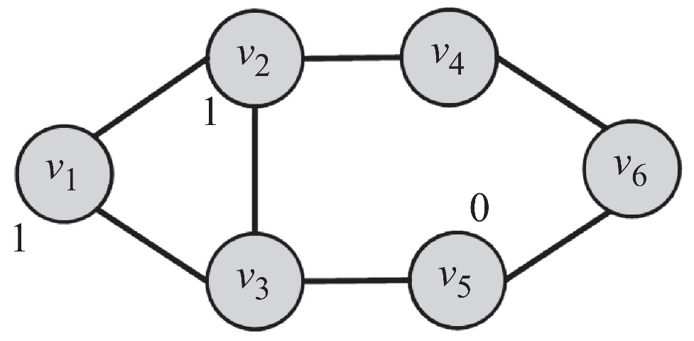
We can assume that \(p(y_i = 1) \approx p(y_i = 1 \mid N(v_i))\), where \(N(v_i)\) denotes \(v_i\)’s neighbors. More specifically, we can let
\[\begin{align*} p(y_i = 1 \mid N(v_i)) = \frac{1}{\lvert N(v_i) \rvert}\sum_{v_j \in N(v_i)} p(y_j=1 \mid N(v_j)). \end{align*}\]We need to compute the probabilities using some order until convergence.
Regression
Linear Regression
Suppose there are a set of observations given by \((\bm{x}^{(1)}, y^{(1)}), \ldots, (\bm{x}^{(m)}, y^{(m)})\) (\(\bm{x}^{(i)} \in \mathbb{R}^{n}\)), and we would like to fit a linear model to describe the relationship between \(\bm{x}\) and \(y\). Denote \(\bm{Y} = (y^{(1)}, \ldots, y^{(m)})^T \in \mathbb{R}^{m}\); \(\bm{X}\in \mathbb{R}^{m\times n}\) is the sample matrix where each row contains an observation. The linear model is given by
\[\begin{align*} \bm{Y} = \bm{XW} + \bm{\epsilon}, \end{align*}\]where \(\bm{W} \in \mathbb{R}^n\) is the model coefficients, and \(\bm{\epsilon}\) denotes error. Usually our goal is to minimize error, i.e. to minimize \(\lVert \bm{\epsilon} \rVert^2 = \lVert \bm{Y} - \bm{XW} \rVert^2\). This is a typical least square problem. With matrix calculus, it can be seen that
\[\begin{align*} &\frac{\partial}{\partial \bm{W}} \lVert \bm{Y} - \bm{XW} \rVert^2\\ &= \frac{\partial}{\partial \bm{W}} (\bm{Y} - \bm{XW})^T(\bm{Y} - \bm{XW})\\ &= \frac{\partial}{\partial \bm{W}} (\bm{Y}^T - \bm{W}^T\bm{X}^T)(\bm{Y} - \bm{XW})\\ &= \frac{\partial}{\partial \bm{W}} (\bm{Y}^T\bm{Y} - \bm{Y}^T\bm{XW} - \bm{W}^T\bm{X}^T\bm{Y} + \bm{W}^T\bm{X}^T\bm{XW})\\ &= -2\bm{X}^T\bm{Y} + 2 \bm{X}^T\bm{X}W. \end{align*}\]Setting it to zero yields
\[\begin{gather*} \frac{\partial}{\partial \bm{W}} \lVert \bm{Y} - \bm{XW} \rVert^2 = 0\\ \Rightarrow -2\bm{X}^T\bm{Y} + 2 \bm{X}^T\bm{X}\bm{W} = 0\\ \Rightarrow \bm{W} = (\bm{X}^T\bm{X})^{-1}\bm{X}^T\bm{Y}. \end{gather*}\]The singular value decomposition (SVD) allows one to compute \(\bm{W}\) efficiently. SVD can express any arbitrary matrix \(\bm{X} \in \mathbb{R}^{m\times n}\) by \(\bm{X}=\bm{U\Sigma V}^T\), where \(\bm{U} \in \mathbb{R}^{m \times m}\), \(\bm{V} \in \mathbb{R}^{n \times n}\) are unitary matrices and \(\bm{\sigma} \in \mathbb{R}^{m\times n}\) is a diagonal matrix. The values on the diagonal are called “singular values”.
Now, given the fact that \(\bm{X}=\bm{U\Sigma V}^T\), and that \(\bm{\Sigma}=\bm{\Sigma}^T\), we can write
\[\begin{align*} \bm{W} &= (\bm{X}^T\bm{X})^{-1}\bm{X}^T\bm{Y}\\ &= (\bm{V}\bm{\Sigma}\bm{U}^T\bm{U\Sigma V}^T)^{-1}\bm{V}\bm{\Sigma}\bm{U}^T\bm{Y}\\ &= (\bm{V}\bm{\Sigma}\bm{\Sigma V}^T)^{-1}\bm{V}\bm{\Sigma}\bm{U}^T\bm{Y}\\ &= (\bm{V}\bm{\Sigma}^2\bm{V}^T)^{-1}\bm{V}\bm{\Sigma}\bm{U}^T\bm{Y}\\ &= (\bm{V}^T)^{-1}\bm{\Sigma}^{-2}V^{-1}\bm{V}\bm{\Sigma}\bm{U}^T\bm{Y}\\ &= \bm{V}\bm{\Sigma}^{-2}\bm{V}^T\bm{V}\bm{\Sigma}\bm{U}^T\bm{Y}\\ &= \bm{V}\bm{\Sigma}^{-2}\bm{\Sigma}\bm{U}^T\bm{Y}\\ &= \bm{V}\bm{\Sigma}^{-1}\bm{U}^T\bm{Y}. \end{align*}\]Since \(\bm{\Sigma}\) is a diagonal matrix, its inverse is very easy to compute (i.e. by replacing the diagonal elements with their reciprocals).
Ridge Regression
In simple linear regression, the model coefficients \(\bm{W}\) is acquired by minimizing \(\lVert \bm{Y} - \bm{XW} \rVert^2\). In this case, we are not restricting the scale of elements in \(\bm{W}\). As a result, some coefficients can be very large, which leads to high variance (i.e. overfitting). In ridge regression, we would like to minimize \(\lVert \bm{Y} - \bm{XW} \rVert^2 + \lambda\lVert \bm{W} \rVert^2\). The second term is called regularization term, its purpose is to control the scale of elements in \(\bm{W}\). The value of \(\lambda > 0\) is a hyperparameter. When \(\lambda \rightarrow \infty\), \(\bm{W} \rightarrow \bm{0}\). When \(\lambda \rightarrow 0\), \(\bm{W}\) will converge to the least square solution.
What is the solution of \(\bm{W}\) in this case? We can use the matrix calculus technique again. It can be seen that
\[\begin{align*} &\frac{\partial}{\partial \bm{W}} \lVert \bm{Y} - \bm{XW} \rVert^2 + \lambda\lVert \bm{W} \rVert^2\\ &= -2\bm{X}^T\bm{Y} + 2 \bm{X}^T\bm{X}W + 2\lambda\bm{W}. \end{align*}\]Setting the partial derivative to zero yields
\[\begin{gather*} -2\bm{X}^T\bm{Y} + 2 \bm{X}^T\bm{X}W + 2\lambda\bm{W} = 0\\ \Rightarrow \bm{X}^T\bm{X}W + \lambda\bm{W}=\bm{X}^T\bm{Y}\\ \Rightarrow (\bm{X}^T\bm{X} + \lambda \bm{I})\bm{W} = \bm{X}^T\bm{Y}\\ \Rightarrow \bm{W} = (\bm{X}^T\bm{X} + \lambda \bm{I})^{-1}\bm{X}^T\bm{Y} \end{gather*}\]A nice property of ridge regression is that it guarantees \((\bm{X}^T\bm{X} + \lambda \bm{I})\) is invertible. First of all, for any given vector \(\bm{z}\), because
\[\begin{align*} \bm{z}^T\bm{X}^T\bm{X}\bm{z} = (\bm{X}\bm{z})^T\bm{Xz} = \lVert \bm{Xz} \rVert^2 \geq 0, \end{align*}\]we know that \(\bm{X}^T\bm{X}\) is positive semi-definite. Suppose \(\bm{v}\), \(c\) are a eigenvector and a eigenvalue of \(\bm{X}^T\bm{X}\), respectively. That is, \(\bm{X}^T\bm{X}\bm{v} = c\bm{v}\). Since \(\bm{X}^T\bm{X}\) is positive semi-definite, we know that \(c \geq 0\). Now, consider
\[\begin{align*} &(\bm{X}^T\bm{X} + \lambda \bm{I})\bm{v}\\ &= \bm{X}^T\bm{X}\bm{v} + \lambda \bm{Iv}\\ &= (c + \lambda)\bm{v}. \end{align*}\]This indicates that \(\bm{v}\) is also an eigenvector of \(\bm{X}^T\bm{X} + \lambda \bm{I}\), and that \(c + \lambda\) is the eigenvalue of \(\bm{X}^T\bm{X} + \lambda \bm{I}\). Because \(\lambda > 0\), it can be seen that the eigenvalues of \(\bm{X}^T\bm{X} + \lambda \bm{I}\) are greater than zero, which indicates that the matrix is positive definite, i.e. the matrix is invertible.
We can still compute \(\bm{W}\) with SVD. It can be seen that
\[\begin{align*} \bm{W} &= (\bm{X}^T\bm{X} + \lambda \bm{I})^{-1}\bm{X}^T\bm{Y}\\ &= (\bm{V}\bm{\Sigma}^2\bm{V}^T + \lambda \bm{V}\bm{V}^T)^{-1}\bm{V}\bm{\Sigma}\bm{U}^T\bm{Y}\\ &= [\bm{V}(\bm{\Sigma}^2 + \lambda\bm{I})\bm{V}^T]^{-1}\bm{V}\bm{\Sigma}\bm{U}^T\bm{Y}\\ &= \bm{V}(\bm{\Sigma}^2 + \lambda\bm{I})^{-1}\bm{V}^T\bm{V}\bm{\Sigma}\bm{U}^T\bm{Y}\\ &= \bm{V}(\bm{\Sigma}^2 + \lambda\bm{I})^{-1}\bm{\Sigma}\bm{U}^T\bm{Y} \end{align*}\]LASSO
LASSO is the acronym for least absolute shrinkage and selection operator. It is very similar to ridge regression, except that the penalty term is \(\ell_1\)-norm. That is, the objective function is given by \(\lVert \bm{Y} - \bm{XW} \rVert^2 + \lambda\lvert \bm{W} \rvert\). Compared to ridge regression, LASSO has a nice property that if an appropriate value of \(\lambda\) is selected, then \(\bm{W}\) will tend to be sparse–many of its elements will be zero. Unfortunately, there is no closed form solution to LASSO. Usually it is solved with quadratic programming techniques.
Clustering
- Goal: to separate data into groups (clusters).
- The problem can be ill-formed. Looking the data at different granularity, there might be different ways to cluster the data. Interpreting the dataset with different semantics can also lead to different clustering results.
\(k\)-means clustering
\(k\)-means clustering is a partitional clustering approach. In \(k\)-means clustering, each cluster is associated with a centroid, and each point is associated to the cluster with the closest centroid. The number of clusters (denoted by \(K\)) needs to be specified. The basic algorithm of \(k\)-means is shown as below.
-
The objective function of \(k\)-means:
\[\sum_{i=1}^{K} \sum_{\bm{x} \in C_i} \lVert \bm{x} - \bm{\mu}_i \rVert^2\](it is possible to use squared cosine distance, squared correlation as well).
- The clustering result is highly influenced by the choice of initial centroids and outliers in data
- Initial centroids are often selected randomly. The algorithm is run multiple times to find the one with smallest objective function.
- The compleity of \(k\)-means is \(O(nKId)\), where \(n\) is the number of data points, \(K\) is the number of clusters, \(I\) is the number of iterations and \(d\) is the number of attributes. It takes linear time with respect to the number of data points.
Spectral clustering
- Idea: suppose the dataset is a graph (or it can be converted into a graph), we can cut the graph into several partitions and assume that these partitions represent clusters.
- The min-cut problem: find a graph partition such that the number of edges between two sets are minimized. This problem can be solved efficiently. However, it usually results in imbalanced cut, which is not very useful.
-
To mitigate the min-cut problem, we can modify the objective function to consider cluster size:
\[\begin{align*} \mbox{Ratio Cut}(P) &= \frac{1}{K}\sum_{i=1}^{K} \frac{\mbox{cut}(P_i, \overline{P_i})}{\lvert P_i \rvert}\\ \mbox{Normalized Cut}(P) &= \frac{1}{K}\sum_{i=1}^{K} \frac{\mbox{cut}(P_i, \overline{P_i})}{\mbox{vol}(P_i)} \end{align*}\]Terms:
- \(\overline{P_i}\): the complement cut set
- \(\mbox{cut}(P_i, \overline{P_i})\): the size of the cut (i.e. the number of edges crossing the cut)
- \(\mbox{vol}(P_i) = \sum_{v\in P_i} d_v\), i.e. the sum of degrees of each node in the set
Examples of ratio cut and normalized cut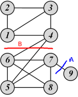
For cut A:
\[\begin{gather*} \mbox{Ratio Cut}(\{1, 2, 3, 4, 5, 6, 7, 8\}, \{9\}) = \frac{1}{2}\left( \frac{1}{1} + \frac{1}{8} \right) = 0.56\\ \mbox{Normalized Cut}(\{1, 2, 3, 4, 5, 6, 7, 8\}, \{9\}) = \frac{1}{2}\left( \frac{1}{1} + \frac{1}{27} \right) = 0.52 \end{gather*}\]For cut B:
\[\begin{gather*} \mbox{Ratio Cut}(\{1, 2, 3, 4\}, \{5, 6, 7, 8, 9\}) = \frac{1}{2}\left( \frac{2}{4} + \frac{2}{5} \right) = 0.45 < 0.56\\ \mbox{Normalized Cut}(\{1, 2, 3, 4\}, \{5, 6, 7, 8, 9\}) = \frac{1}{2}\left( \frac{2}{12} + \frac{2}{16} \right) = 0.15 < 0.52 \end{gather*}\]Therefore, both ratio cut and normalized cut suggest that cut B is a better cut.
- Reformulating the ratio cut in matrix format:
- Let \(\bm{X}_{ij} = 1\), when node \(i\) is member of cluster \(j\); 0 otherwise.
- Let \(\bm{A}\) be the similarity matrix: \(A_{ij}=1\) if there is an edge between node \(i\) and node \(j\); 0 otherwise. Let \(D = \mbox{diag}(d_1, d_2, \ldots, d_n)\) be the diagonal degree matrix. It is obvious that \(d_i = \sum_{j} A_{ij}\).
- The \(i\)th entry on the diagonal of \(\bm{X}^T\bm{A}\bm{X}\) is the number of edges that are inside cluster \(i\).
- The \(i\)th element on the diagonal of \(\bm{X}^T\bm{D}\bm{X}\) is the number of edges that are connected to the members of cluster \(i\).
- The \(i\)th element on the diagonal of \(\bm{X}^T(\bm{D}-\bm{A})\bm{X}\) is the number of edges in the cut that separates the community \(i\) from other nodes.
For ratio cut, it can be seen that
\[\begin{align*} \mbox{Ratio Cut}(P) &= \frac{1}{K}\sum_{i=1}^{K} \frac{\mbox{cut}(P_i, \overline{P_i})}{\lvert P_i \rvert}\\ &= \frac{1}{K}\sum_{i=1}^{K} \frac{\bm{X}_i^T (\bm{D}-\bm{A}) \bm{X}_i}{\bm{X}_i^T\bm{X}_i}\\ &= \frac{1}{K}\sum_{i=1}^{K} \hat{\bm{X}}_i^T (\bm{D}-\bm{A}) \hat{\bm{X}}_i, \end{align*}\]where \(\hat{\bm{X}}_i = \bm{X}_i/(\bm{X}_i^T\bm{X}_i)^{1/2}\).
-
As it turns out, both ratio cut and normalized cut can be reformulated as
\[\min_{\hat{\bm{X}}} \operatorname{Tr}(\hat{\bm{X}}^T \bm{L} \hat{\bm{X}}),\]where
\[\begin{align*} \bm{L} = \begin{cases} \bm{D} - \bm{A}, & \mbox{ratio cut Laplacian}\\ \bm{I} - \bm{D}^{-1/2}A\bm{D}^{-1/2}, &\mbox{normalized cut Laplacian} \end{cases}. \end{align*}\]Solving this problem directly is NP Hard. If we perform a relaxation, that is, we set \(\hat{\bm{X}}^T\hat{\bm{X}} = \bm{I}\), then the optimal solution is given by the top eigenvectors of \(\bm{L}\) with the smallest eigenvalues. Then, we can run \(k\)-means clustering on the eigenvector to retrive the clusters.
Evaluation
-
Goal: to determine the effectiveness of a clustering algorithm.
-
Types of measures:
-
External index: Used to measure the extent to which cluster labels match externally supplied class labels (e.g. entropy)
-
Internal index: Used to measure the goodness of a clustering structure without respect to external information (e.g. Sum of Squared Error (SSE))
-
Relative Index: Used to compare two different clusterings or clusters. Often an external or internal index is used for this function, e.g., SSE or entropy
-
Internal measures
Cohesion and Separation
-
Cluster cohesion is the sum of the weight of all links within a cluster. It is measured by the within cluster sum of squares.
\[\begin{align*} WSS = \sum_i \sum_{\bm{x} \in C_i} (\bm{x} - \bm{\mu}_i)^2 \end{align*}\] -
Cluster separation is the sum of the weights between nodes in the cluster and nodes outside the cluster. It is measured by the between cluster sum of squares.
\[BSS = \sum_i \lvert C_i \rvert (\bm{\mu} - \bm{\mu}_i)^2,\]where \(\bm{\mu}\) is the centroid of the entire dataset.
-
It can be proved that \(WSS + BSS\) is some constant. That is, minimizing cluster cohesion maximizes cluster separation.
Silhouette Coefficient
Silhouette coefficient combines ideas of both cohesion and separation, but for individual points, as well as clusters and clusterings.
For an individual point \(i\),
-
calculate \(a\)=average distance of \(i\) to the points in its cluster
-
calculate \(b\)=the smallest mean distance of \(i\) to all points in any other cluster, to which \(i\) is not a member.
-
The silhouette coefficient of a point is then given by
\[\begin{align*} s = \frac{(b-a)}{\max(a, b)}. \end{align*}\] -
The range of \(s\) is typically between 0 and 1. The closer to 1, the better.
-
It is possible to compute the average silhouette coefficient for a cluster or clustering.
Big Data
This part of the lecture is based on Mining of Massive Datasets, which targets machine learning/data retrieval on huge datasets that might not fit in any type of memory medium.
MapReduce
- The new trend in big data processing: using clusters that are made up of inexpensive computers instead of one supercomputer.
- MapReduce is a computation model that can be easily implemented on clusters. It is resistant to node errors, which is common on such clusters.
- Within a cluster, the greatest cost is communication. Sometimes computational complexity is not the major time factor.
A MapReduce algorithm consists of two parts: a map function and a reduce function.