PyCG 7: Simple Ray Tracing

Ray tracing is a way of rendering photo-realistic photos. I made use of this concept in this post to compute the image of projecting on a spherical screen. This time, let us build a simple ray tracer with Python. This time, OpenGL is not needed.

The ray tracing algorithm

The idea behind ray tracing is straightforward: the light source gives out an infinite amount of rays, which interacts with the objects in the scene. Eventually, some of the rays will enter the camera and be captured as image. However, if the algorithm is implemented in this way, it is very inefficient because only a very small proportion of the rays will be seized by the camera. This means that most of the computation is useless. To avoid this problem, ray tracing algorithms will try to render the scene in an reversed order (as shown in the figure below): for every pixel of the image, a primitive ray will be generated and tested against the rest of the objects in the scene. If an intersection is found, a shadow ray will be generated to find out if it is inside the shadow of another object or it is directed radiated by the light source. By doing this, we save a huge amount of computation.

As a matter of fact, ray tracing can be one of the easiest rendering algorithms to implement. It is nontrivial to render some simple geometry objects, for example - lines on screen with scanline rendering. The pseudocode of the ray tracing algorithm can be seen as below:

\begin{algorithm}
\begin{algorithmic}

\FUNCTION{RayTracing}{$primitiveRay, targetPixel, strength, depth$}
    \IF{$strength < strengthThreshold$ \OR $depth > maxDepth$}
    \RETURN
    \ENDIF

    \STATE{find the intersection between $primitiveRay$ and the object that is nearest to the eye}

    \IF{there is an intersection}
        \STATE\COMMENT{remember to add a small offset to the shadow ray to avoid self-intersection}
        \STATE{test if the shadow ray intersects with any objects in the scene}
        \IF{the shadow ray does not intersect with anything else}
            \STATE{update $targetPixel$ with color values computed from shading model}
            \STATE{$reflectionRay$ = the computed reflection ray}
            \STATE{$newStrength$ = the strength of the reflection ray (computed according to $strength$)}
            \STATE\CALL{RayTracing}{$reflectionRay, targetPixel, newStrength, depth + 1$}
        \ENDIF
    \ENDIF

\ENDFUNCTION

\end{algorithmic}
\end{algorithm}

We can run this method for each pixel in the image to get the result.

The computation of intersection and normal

I have implemented two types of objects in the demo, namely triangles and spheres. They are geometry objects with simple mathematical expressions, which can be dealt with very easily.

1. Triangle

   A triangle can be defined by its three vertices \(\bm{p}_1\), \(\bm{p}_2\), \(\bm{p}_3\), which should be ordered counterclockwise to ensure a correct surface normal direction. The surface normal \(\bm{n}\) is given by

   \[\mathrm{normalize}\left[\left( \bm{p}_2 - \bm{p}_1 \right) \times \left(\bm{p}_3 - \bm{p}_1\right)\right],\]

   where “\(\times\)” denotes cross product. The equation of its corresponding plane is \((\bm{x} - \bm{p}_1) \cdot \bm{n} = 0\). Assume that there is a ray given by \(\bm{o} + t\bm{d}\), combining these two equations gives

   \[\begin{gather*} (\bm{o} + t\bm{d} - \bm{p}_1) \cdot \bm{n} = 0\\ t = \frac{\bm{p}_1 \cdot \bm{n} - \bm{o} \cdot \bm{n}}{\bm{d} \cdot \bm{n}} \end{gather*}\]

   The intersection \(\bm{w}\) is the value of \(\bm{o} + t\bm{d}\). Now we need to decide if the intersection is in the triangle. To do this, we need to first form a matrix \(\bm{M}\), where

   \[\bm{M} = \begin{pmatrix} \left( \bm{p}_2 - \bm{p}_1 \right)_x & \left( \bm{p}_3 - \bm{p}_1 \right)_x & \bm{n}_x\\ \left( \bm{p}_2 - \bm{p}_1 \right)_y & \left( \bm{p}_3 - \bm{p}_1 \right)_y & \bm{n}_y\\ \left( \bm{p}_2 - \bm{p}_1 \right)_z & \left( \bm{p}_3 - \bm{p}_1 \right)_z & \bm{n}_z. \end{pmatrix}\]

   we can compute the coordinates of \(\bm{w}\) with the sides of the triangle as base by

   \[\bm{w'} = \bm{M}^{-1}(\bm{w} - \bm{p}_1).\]

   The intersection is in the triangle i.f.f. \(\bm{w'}_x > 0, \bm{w'}_y > 0\) and \(\bm{w'}_x + \bm{w'}_y < 1\).

2. Sphere

   The equation of a sphere is given by \(\lVert \bm{x} - \bm{p}_0 \rVert = r\), where \(\bm{p}_0\) is the center and \(r\) is the radius. Using the same line equation, it yields

   \[\begin{gather*} \lVert \bm{o} + t\bm{d} - \bm{p}_0 \rVert = r\\ \lvert \bm{o} \vert^2 + t^2 \lvert \bm{d} \rvert^2 + \lvert \bm{p}_0 \rvert^2 + 2t \bm{o} \cdot \bm{d} - 2t\bm{d} \cdot \bm{p}_0 - 2\bm{o} \cdot \bm{p}_0 = r^2\\ t^2 \lvert \bm{d} \rvert^2 + t \left[ 2\left( \bm{o}\cdot\bm{d} - \bm{d}\cdot\bm{p}_0 \right) \right] + \lvert \bm{o} \vert^2 + \lvert \bm{p}_0 \rvert^2 - 2\bm{o} \cdot \bm{p}_0 - r^2 = 0, \end{gather*}\]

   which is simply a quadratic equation with

   \[\begin{equation*} \left\{ \begin{aligned} a &= \lvert \bm{d} \rvert^2\\ b &= 2\left( \bm{o}\cdot\bm{d} - \bm{d}\cdot\bm{p}_0 \right)\\ c &= \lvert \bm{o} \vert^2 + \lvert \bm{p}_0 \rvert^2 - 2\bm{o} \cdot \bm{p}_0 - r^2. \end{aligned} \right. \end{equation*}\]

   The determinant \(\Delta = b^2 - 4 ac\) indicates if there is an intersection between the ray and the sphere. If solution exists, we choose the one with smaller \(t\) value because it is closer to the eye.

The object oriented approach

Graphics programs are probably one of the best type of programs that fit with the object-oriented paradigm. That is mainly because the objects we interacts with (e.g. triangles, spheres) all share similar interfaces. For example, they must all provide intersect method to calculate intersection, normal method to compute surface normal and shade method to acquire color under the specific lighting configuration. With OOP, we can let all graphics objects inherit from some base class that has these common methods, which will greatly reduce the difficulty of designing the program. In Python, because of dynamic typing, I did not use inheritance explicitly.

Demo

The source code can be found on GitHub. The core logic that affects the scene is this part in main.py:

# declares the ray tracing config
config = RayTracingConfig()
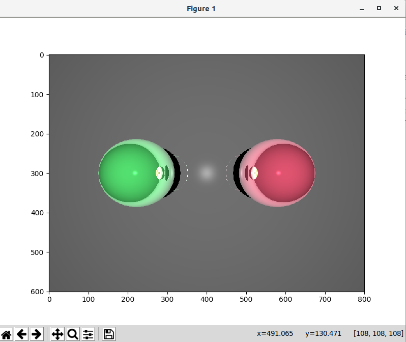
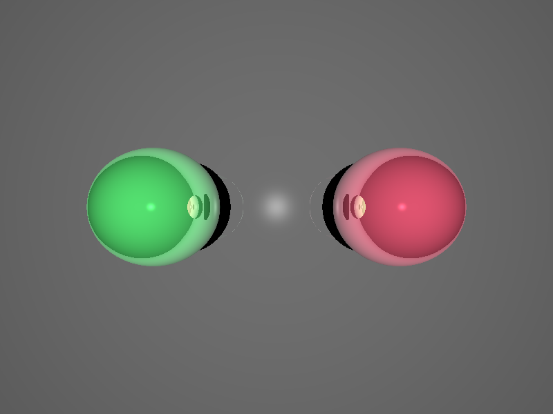
config.imageShape = (600, 800)
config.cameraOrigin = np.asarray([0.0, 0.0, 4.0])
config.cameraUp = np.asarray([0.0, 1.0, 0.0])
config.cameraFront = np.asarray([0.0, 0.0, -1.0])
config.cameraFocalLength = 0.1
config.lightColor = np.asarray([1.0, 1.0, 1.0], np.float32)
config.lightPos = np.asarray([0.0, 0.0, 10.0])

# object1: a sphere
sphere1 = Sphere(np.asarray([-2.0, 0.0, 0.0], np.float), 1.0)
sphere1.shadeParam.color = np.asarray([0.3, 0.8, 0.4], np.float32)
# object1: another sphere
sphere2 = Sphere(np.asarray([2.0, 0.0, 0.0], np.float), 1.0)
sphere2.shadeParam.color = np.asarray([0.8, 0.3, 0.4], np.float32)

p1 = np.asarray([-16.0, 16.0, -2.0])
p2 = np.asarray([-16.0, -16.0, -2.0])
p3 = np.asarray([16.0, -16.0, -2.0])
p4 = np.asarray([16.0, 16.0, -2.0])

# object3: background triangle 1
tri1 = Triangle(p1, p2, p3)
tri1.shadeParam.reflectionStrength = 0.3
tri1.shadeParam.color = np.asarray([0.4, 0.4, 0.4], np.float32)

# object4: background triangle 2
tri2 = Triangle(p1, p3, p4)
tri2.shadeParam.color = tri1.shadeParam.color
tri2.shadeParam.reflectionStrength = tri1.shadeParam.reflectionStrength

# the scene (array of all objects)
objects = [
    sphere1,
    sphere2,
    tri1,
    tri2
]

# how many processes in the process pool
concurrency = 10

To facilitate the computation, I use the ThreadPool class to distribute the computation across CPU cores. The result is shown with matplotlib. On my computer (Intel Core i7-8700K), it takes around 20 seconds to render an \(800 \times 600\) image.